2.5 quintillion bytes of data are produced every day! Consider how much we can deduce from that and what conclusions we can draw. Wait! But, how do we deal with such a massive amount of data?
Not to worry; the Pandas library is your best friend if you enjoy working with data in Python.
But what exactly is Pandas, and why should we use it?
Pandas is a Python library used for working with large amounts of data in a variety of formats such as CSV files, TSV files, Excel sheets, and so on. It has functions for analyzing, cleaning, exploring, and modifying data. Pandas can be used for a variety of purposes, including the following :
Pandas enable the analysis of large amounts of data and drawing conclusions based on statistical theories.
Real-world data is never perfect and requires a lot of work; the Pandas library makes this work easier and faster, making datasets more relevant and cleaner.
It has a robust feature set you can apply to your data to customize, edit, and pivot it to your liking. This makes getting the most out of your data a lot easier.
It also allows you to represent data in a very streamlined way. This aids in data analysis and the ability to comprehend.
These are just a few of the Pandas library’s many benefits. So, let us delve deep into this library and bring all the benefits listed to live! It sounds interesting, don’t you think? Learning about the Pandas Library will pique your interest.😁
Pandas Installation
Before you can learn about the Pandas library, you must first install it on your system. To do so, install Anaconda and, once installed, enter the following code into your Anaconda Prompt.
conda install pandas
Now that we’ve installed Pandas on our system, let’s look at the data structures it contains.
Data Structures In Pandas
The Pandas library deals with the following data structures :
Pandas Data Frame :
Whenever there is a dataset with at least two columns and any number of records(rows) then it is known as a Data frame.
Pandas Series :
Whenever there is a dataset with just a single column with any number of records (rows) then it is known as a Series.
IMAGE 1
Importing The Pandas Library
Before learning and using the functionalities of Pandas, it is necessary to import the Pandas libraryPandas library first. We do so by writing the following code into our Jupyter notebook :
import pandas as pd
Note : “pd” is used as an alias so that the Pandas package can be referred to as “pd” instead of “pandas”.
Now that we have installed Pandas and also imported it into our Jupyter notebook, we can now explore the different functionalities of Pandas.
Importing Data
Before working on data, we have to first import it. The Pandas library has a variety of commands for dealing with different forms of data. We will be learning about one such command which deals with CSV files.
1. read_csv()
The pd.read_csv() command is used to read a CSV file into data frame.
Before working with your data, it is necessary to know about your data properly. Pandas help you in doing so :
1. head() and tail()
The above output is not very intriguing to watch. Let us try looking at only first or last few records of our dataset. We can do so by using the following Pandas commands.
The df.head() command helps us view our dataset’s top 5 (default value) records. If you want to view more than 5, you can do so by typing – df.head(n) where n is the number of records you want to view.
df.head()
The df.tail() command helps us view our dataset’s last 5 (default value) records. If you want to view more than 5, you can do so by typing – df.tail(n) where n is the number of records you want to view.
df.tail()
2. shape
The df.shape command provides you with the number of rows and columns in your dataset.
df.shape()
3. info()
The df.info() command prints the information about our dataset, including columns, datatypes of columns, non-null values, and memory usage.
df.info()
4. describe()
The df.describe() command calculates a summary of statistics for the data frame columns. This function returns the count, mean, standard deviation, and interquartile range (IQR) values.
df.describe()
5. nunique()
The df.nunique command returns the number of unique entries in each column.
df.nunique()
Selection Of Data
You often do not want to work with only a subset of the entire dataset. In such cases, use the following commands:
1. df[col]
The df[col] command returns the column with the specified label as series.
# selecting the column 'title'
df['title']
2. df[[col1,col2]]
The df[[col1, col2]] returns columns as a data frame.
# selecting the columns 'title' and 'mediaType'
df[['title', 'mediaType']]
3. loc[ ]
The df.loc[ ] command helps you access a group of rows and columns. loc is label-based, which means that you have to specify rows and columns based on their row and column labels. It includes the ends, i.e., df.loc[0:4] will return all the rows from 0-4(included).
# selecting all the rows from 0-4 and the associated columns
df.loc[ :4]
# selecting all the rows and the column named 'title'
df.loc[: , 'title']
# selecting all the rows from 1-5 and the columns named 'title' and 'rating'
df.loc[1:5, ['title', 'rating'] ]
# selecting all the rows and columns with entries having rating > 4.5
df.loc[df['rating'] > 4.5]
4. iloc[ ]
The df.iloc[ ] command also helps you access a group of rows and columns. Still, unlike loc, iloc is integer position-based, so you have to specify rows and columns by their integer position values. It excludes the ends, i.e., df.iloc[0:4] will return all the rows from 0-3 as 4 is excluded.
# selecting all the rows from 0-4(excluded) and the associated columns
df.iloc[0:4]
# selecting all the rows and columns
df.iloc[: , :]
# selecting all the rows and columns from 0-4(excluded)
df.iloc[0:4, 0:4]
# selecting all the rows from 0-10(excluded) and the 0th, 2nd, and 5th columns
df.iloc[ 0:10, [0, 2, 5] ]
# selecting the 3rd, 4th, and 5th rows and the 0th and 2nd columns
df.iloc[[3, 4, 5], [0, 2]]
Filter, Sort & Groupby
When working with datasets, you will encounter circumstances when you need to sort, filter, or even group your data to make it easier to understand. The commands listed below will be your helping hands in this :
1. df[df[col] operator number]
The df[df[col] operator number] command helps you easily filter out data.
# selecting all the records where column 'watched' > 1000
df[df['watched] > 1000]
# selecting all the records where column 'watched' < 100
df[df['watched'] < 100]
# filtering out with multiple conditions.
# selecting all the records where 'watched' > 1000 and 'eps' = 10
df[(df['watched'] > 1000) & (df['eps'] == 10)]
2. sort_values()
The df.sort_values() command helps in sorting your data in ascending or descending manner.
# sorting the values of the column 'eps' in ascending manner(default)
df.sort_values('eps')
# sorting the values of the column 'eps' in descending manner
df.sort_values('eps' , ascending = False)
# sorting multiple columns in ascending and descending manner
# sorting the column 'eps' in ascending order and 'duration' in descending order
df.sort_values(['eps', 'duration'], ascending = [True, False])
3. Groupby()
The df.groupby() command helps split data into separate groups and lets you perform functions on these groups.
# the below code means we want to analyze our data by different "eps" values.
# the below code returns a DataFrameGroupBy object
df_groupby_eps = df.groupby('eps')
df_groupby_eps
# using the size() attribute
# it will display the group sizes [there are 7307 animes having only 1 episode and so on]
df_groupby_eps.size()
# using the get_group() attribute
# it will retrieve one of the created groups
# it will display the anime that has 500 episodes
df_groupby_eps.get_group(500.0)
# making use of aggregate functions to compute on grouped data
# applying the mean function on the grouped data
df_groupby_eps.mean()
# using the agg() function
# we can apply different aggregate functions.
# the below code will display the maximum and minimum rating of animes which are grouped by their votes.
df.groupby('votes').rating.agg(['max', 'min])
Data Cleaning
If your elders have warned you about how the real world is not what we think it is, how it is messy and uninterpretable, then let me add something more to it. Real-world data is just the same: messy and uninterpretable. You first have to clean the data to get the most out of your data and infer meaningful insights. And as I mentioned, Pandas is your best friend, so well, your best friend has got it all covered.
1. isnull()
The df.isnull() command checks for all the null values in your dataset.
# checking for null values
# it will return the dataset with the entries as True / False where True means that this cell has a null value and False means that this cell does not has a null value.
df.isnull()
# we can use the sum() function with isnull()
# it will return the sum of null values for each column
df.isnull().sum()
2. notnull()
The df.notnull() command is just the opposite of df.isnull() command. This command will check for the non-null values in the dataset.
# returns the dataset with entries as True/False where True means not having a null value and False means having a null value.
df.notnull()
# using the sum() function
# it will return the sum of all the non null values for each column.
df.notnull().sum()
3. dropna()
The dropna() command drops the rows/columns with missing entries.
# dropping all the rows with missing values
df.dropna()
# using the "axis" parameter
# "axis = 0" (default) means Row and "axis = 1" means Column
# dropping all the columns with missing entries
df.dropna(axis = 1)
# using the "how" parameter
# how = "any" means dropping rows/columns having "ANY" missing entries.
# how = "all" means dropping rows/columns having "ALL" missing entries.
# dropping the columns having any missing values.
df.dropna(axis = 1, how = 'any')
# using the "thresh" parameter
# it specifies how many non-null values a row or column must have so as to not be dropped
# keeping only the columns with at least 14000 non-null values
df.dropna(axis = 1, thresh = 14000)
# using the "subset" parameter
# it is used for defining in which columns to look for missing values
# dropping all the rows where the "duration" column is NaN
df.dropna(subset = ['duration'])
NOTE : The dropna() and fillna() commands returns a copy of your object rather than the actual object. To update your object , you need to specify the value of the inplace parameter as True. Don’t worry, the inplace parameter is covered below.
3. fillna()
The df.fillna() command does exactly what its name implies: it fills in the missing entries with some value.
# filling the NaN values with some user specified value
df.fillna(value = "Not Specified")
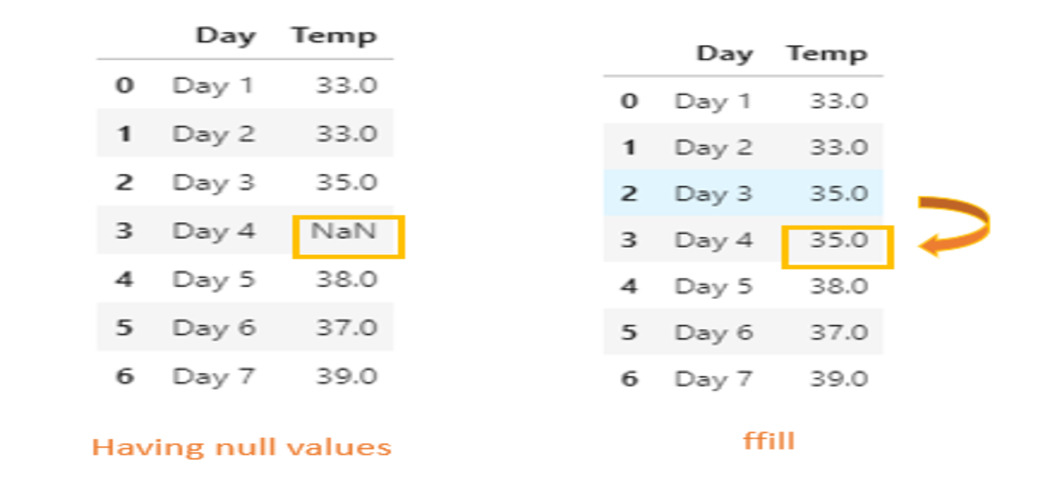
using the “method” parameter
it specifies how shall we fill the missing values
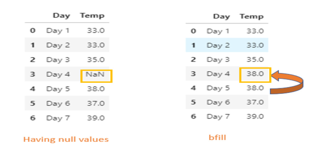
method = ‘ffill’/ ‘bfill’
“ffill” stands for forward fill
“bfill” stands for backward fill
HOW THE FFILL METHOD WORKS
HOW THE BFILL METHOD WORKS
# executing the ffill method
df.fillna(method = 'ffill')
# executing the bfill method
df.fillna(method = 'bfill')
# using the "inplace" parameter
# The 'inplace = True' argument means that the data frame has to make changes permanent.
# If you use 'inplace = False' (default), you basically get back a copy
# This is before using 'inplace = True'
df.dropna().head(2)
df.isnull().sum()
df.fillna(value = 1).head(2)
df.isnull().sum()
# after using 'inplace = True'
df.dropna(inplace = True)
df.isnull().sum()
NOTE: As all the rows with missing values are dropped, there is no need to use fillna().
4. rename()
The df.rename() command helps us in altering axes labels.
# renaming the 'eps' column as 'Episodes'
df.rename(columns = {'eps' : 'Episodes'})
Question: Can you guess why the records start from 149 instead of 0?
Creating Test Objects
You don’t necessarily need to use pre-existing datasets; instead, you can generate your own test objects and run a range of commands to explore this library further. You are covered in that by the following commands :
1. DataFrame() & Series()
The pd.DataFrame() command helps you create your own data frame with ease.
The pd.Series() command helps you create your own series with ease.
Pandas’ ability to apply statistical techniques to data is beneficial since it improves the analysis and interpretation of the data. The commands listed below assist us in achieving that :
1. mean() & median()
The df.mean() and df.median() commands returns the mean and median(respectively) of all columns.
df.mean()
df.median()
2. corr()
The df.corr() command returns the correlation between columns.
# correlation can be defined as a relationship between variables.
# it lies between -1 and 1 (inclusive of both the values)
df.corr()
3. std()
The df.std() command returns the standard deviation of all the columns.
df.std()
4. max() & min()
The df.max() and df.min() commands returns the highest and lowest value in each columns.
df.max()
df.min()
Combining Data Frames
Combining datasets is necessary when you have multiple datasets yet want to study all their data simultaneously. The commands listed below can be useful in this scenario :
1. concat()
The pd.concat() command lets you combine data across rows or columns.
# using the "axis" parameter
pd.concat([df2,df3,df4], axis = 1)
Conclusion
Pandas is one of the most useful and user-friendly data science and machine learning libraries. It aids in deriving meaningful insights from various types of datasets. It has outstanding features that, if properly understood, can be useful when working with data and speed up your process. Do not stop learning about this incredible library here because the Pandas library has many more interesting functionalities with which you can infer insights from data in minutes!
Thank you for reading!😊
The media shown in this article is not owned by Analytics Vidhya and is used at the Author’s discretion.
We use cookies on Analytics Vidhya websites to deliver our services, analyze web traffic, and improve your experience on the site. By using Analytics Vidhya, you agree to our Privacy Policy and Terms of Use.Accept
Privacy & Cookies Policy
Privacy Overview
This website uses cookies to improve your experience while you navigate through the website. Out of these, the cookies that are categorized as necessary are stored on your browser as they are essential for the working of basic functionalities of the website. We also use third-party cookies that help us analyze and understand how you use this website. These cookies will be stored in your browser only with your consent. You also have the option to opt-out of these cookies. But opting out of some of these cookies may affect your browsing experience.
Necessary cookies are absolutely essential for the website to function properly. This category only includes cookies that ensures basic functionalities and security features of the website. These cookies do not store any personal information.
Any cookies that may not be particularly necessary for the website to function and is used specifically to collect user personal data via analytics, ads, other embedded contents are termed as non-necessary cookies. It is mandatory to procure user consent prior to running these cookies on your website.
.jpg)
.jpg)
.jpg)
.jpg)
.jpg)
.jpg)
.jpg)
.jpg)
.jpg)
.jpg)
.jpg)
.jpg)
.jpg)
.jpg)
.jpg)
.jpg)
.jpg)
.jpg)
.jpg)
.jpg)
.jpg)
.jpg)
.jpg)
.jpg)
.jpg)
.jpg)
.jpg)
.jpg)
.jpg)
.jpg)
.jpg)
.jpg)
.jpg)
.jpg)
.jpg)
.jpg)
.jpg)
.jpg)
.jpg)
.jpg)
.jpg)
.jpg)
.png)
.jpg)
.jpg)
.jpg)
.jpg)
.jpg)
.jpg)
.jpg)
.jpg)
.jpg)
.jpg)


