Identifying and Dealing with Multicollinearity and Heteroscedasticity

This article was published as a part of the Data Science Blogathon.

Introduction

Heteroscedasticity is an error term that implies unequal scattered distribution of residuals in a regression analysis. Heteroscedasticity mainly occurs due to outliers in the data. Besides, Multicollinearity indicates a high correlation between independent variables. Multicollinearity may affect the performance of the regression models. Even some Machine Learning algorithms are too sensitive to Multicollinearity. That means these ML algorithms do not deal with Multicollinearity and produce poor results. Therefore, we need to tackle the Multicollinearity by ourselves with regression models.

This article will discuss Heteroscedasticity and Multicollinearity in detail with Python implementation. We will use the Moscow Apartments listing dataset from Kaggle for Heteroscedasticity and WeatherAUS data for Multicollinearity analysis.

You can use any platform for Python implementation, like Google Colaboratory or Jupyter Notebook. So, get ready to get your hands dirty in buggy war.

First, we import all the necessary libraries and data into the Jupyter notebook.

## Importing necessary libraries
import pandas as pd  ## Data exploration and manipulation
import numpy as np  ## Mathematical calculation
import matplotlib.pyplot as plt  ## Visualizing the data
import seaborn as sns   ## Statistical Analysis
weather_aus = pd.read_csv('weatherAUS.csv')   ## Loading the dataset
weather_aus.head()   ## showing top 5 rows

Now, let’s dive into these concepts one by one with our notebook:

What is Multicollinearity

Multicollinearity occurs when the dataset has two or more highly correlated independent variables. Although This phenomenon does not affect the model performance, it does affect the model interpretability. We may find two variables in feature importance have a high correlation even though only one of them is enough.

For example, age and birth year, weight and height, salary and monthly income, etc.

Cause of Multicollinearity

There are various reasons for Multicollinearity, and a few of them are as follows:

• Poor experiment design, data manipulation error, or incorrect data observations.

For example, we interchange the data for some rows of income and salary columns.

• Creating a new variable that is dependent on other available variables. For instance, if the income variable is with monthly salary and other incomes.
• Having identical variables in the dataset. For example, If the age variable is taken as year and in months too.
• Including both columns in the dataset while creating dummy variables from categorical features will cause Multicollinearity.

These are some reasons for Multicollinearity in the dataset, although there are more reasons too.

Detecting the Multicollinearity

We must detect Multicollinearity before building a predictive model since we may not be able to differentiate between the individual contribution of each independent variable and the relation with the dependent variable.

import statsmodels.api as sm              ## Performing statistical methods
from statsmodels.stats.outliers_influence import variance_inflation_factor    ## For checking Multicollinearity
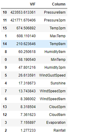
## Checking Multicollinearity
vif_info = pd.DataFrame()   ## Creating an empty data frame
vif_info['VIF'] = [variance_inflation_factor(df.values, i) for i in range(df.shape[1])]   ## Creating a new column with VIF values
vif_info['Column'] = df.columns  ## A new column with all the independent variables
vif_info.sort_values('VIF', ascending=False)   ## Sorting the data in descending order

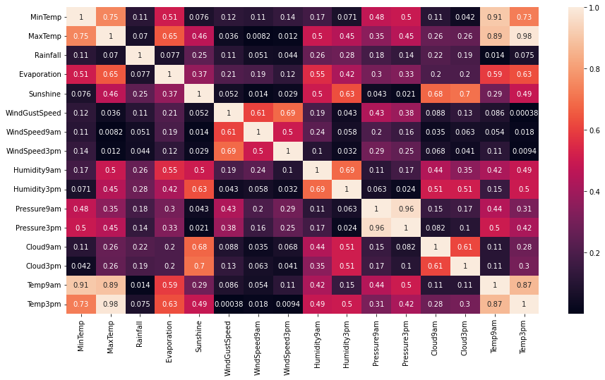
plt.figure(figsize = (15,8))   ## Size of the figure
sns.heatmap(df.corr().abs(), annot = True)   ## Heatmap for the correlation

Handling the Multicollinearity

We must remove the Multicollinearity from the dataset after detecting it. There are various methods to fix Multicollinearity, and we will discuss two of the most effective techniques:

Creating new features

This method is the most significant tactic to remove Multicollinearity. We will create some new features using highly correlated variables and will drop the columns with high correlation. Then we can use these new features to identify Multicollinearity and model building.

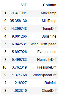
## Creating new features
df['TempDiff'] = df['Temp3pm'] - df['Temp9am']   
df['HumidityDiff'] = df['Humidity3pm'] - df['Humidity9am']
df['CloudDiff'] = df['Cloud3pm'] - df['Cloud9am']
df['WindSpeedDiff'] = df['WindSpeed3pm'] - df['WindSpeed9am']
df['PressureDiff'] = df['Pressure3pm'] - df['Pressure9am']
## Dropping highly correlated features
X = df.drop(['Temp3pm', 'Temp9am', 'Humidity3pm', 'Humidity9am', 'Cloud3pm', 'Cloud9am', 'WindSpeed3pm', 'WindSpeed9am', 'Pressure3pm', 'Pressure9am'], axis=1)
X.head()  ## Checking first 5 rows

## Checking Multicollinearity again

vif_info = pd.DataFrame()
vif_info['VIF'] = [variance_inflation_factor(X.values, i) for i in range(X.shape[1])]
vif_info['Column'] = X.columns
vif_info.sort_values('VIF', ascending=False)

Removing features

We can also remove the highly correlated independent variables from the dataset, although not recommended due to the risk of essential information loss.

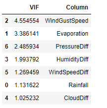
## Removing the highly correlated features
X_new = X.drop(['MaxTemp', 'MinTemp', 'TempDiff', 'Sunshine'], axis=1)
## Multicollinearity checking
vif_info = pd.DataFrame()
vif_info['VIF'] = [variance_inflation_factor(X_new.values, i) for i in range(X_new.shape[1])]
vif_info['Column'] = X_new.columns
vif_info.sort_values('VIF', ascending=False)

Heteroscedasticity

Heteroscedasticity is a phenomenon that occurs due to the presence of outliers in the dataset. The meaning of Heteroscedasticity is unequal scattered distribution. In regression analysis, the residuals spread over the measured values range with systematic change. This error distribution becomes unequally scattered and is known as Heteroscedasticity.

Ordinary Least Square, or OLS, expects the residuals drawn from a random population with constant variance.

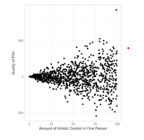
Scatter plot between predicted and residuals

You can identify the Heteroscedasticity in a residual plot by looking at it. If the shape of the graph is like a fan or a cone, then it is Heteroscedasticity. Another indication of Heteroscedasticity is if the residual variance increases for fitted values.

Types of Heteroscedasticity

There are two types of Heteroscedasticity that we may generally encounter:

1. Pure Heteroscedasticity – When we use proper independent features, the residual plot shows the non-non-constant variance. In other words, we observe unequal residual variance despite specifying the correct model.
2. Impure Heteroscedasticity – This scenario is typical where we specify an incorrect model, and the number of input features also gets the unequal residual variance.

Reason for Heteroscedasticity

Heteroscedasticity occurs due to changes in error variance. If the dataset has a wide range of values with a significant difference between the minimum and the maximum observed values. Hence we can say that Heteroscedasticity is a problem because of the dataset. There are various examples of Heteroscedasticity in real life, such as retail eCommerce sales during the last 30 years. There were very few e-commerce customers ten years ago; hence the observed values would be less.

On the other hand, e-commerce sales have gone up within the last decade. Consequently, we will find a wide range of values in this scenario. Thus, we may face a Heteroscedasticity problem in the dataset.

The cross-sectional datasets are more likely to have Heteroscedasticity. For example, the income of all Indian workers will cause Heteroscedasticity due to differences in their salaries or wages. However, if we were to analyze the salaries of one segment, say Developers, you may not find a broad range of values.

Detecting Heteroscedasticity

Now that we have understood what Heteroscedasticity is and why it occurs. We will discuss how to identify and remove Heteroscedasticity from the dataset. The method that will detect Heteroscedasticity is the Het-White Test.

We have performed the Het-White test on the Moscow Apartment Listing dataset we used for Multicollinearity testing. The Het-White test is already available in the Statsmodel library of Python. First, we make two hypotheses: Null (H0) and Alternate (H1).

H0: The dataset has homoskedasticity.

H1: The dataset does not have homoskedasticity but Heteroscedasticity.

The test returns values for ‘Lagrange Multiplier statistic’, ‘LM test’s p-value’, ‘F-statistic’, and ‘F-test’s p-value’. If the P-value output is less than 0.05. Then we reject the null hypothesis. We have implemented the test in Python as presented below:

from statsmodels.stats.diagnostic import het_white
from statsmodels.compat import lzip
from patsy import dmatrices
expr = 'price~ repair+ year_built_empty+house_age+closest_subway+dist_to_subway+sg+subway_dist_to_center+h3+agent_offers+subway_offers+address_offers+rooms+footage+floor+max_floor+first_floor+last_floor+AO+hm' 
model = OLS.from_formula(expr, data=moscow_df).fit()
p = model.params
y, X = dmatrices(expr, moscow_df, return_type='dataframe')
keys = ['Lagrange Multiplier statistic:', 'LM test's p-value:', 'F-statistic:', 'F-test's p-value:']
results = het_white(model.resid, model.model.exog)
lzip(keys, results)

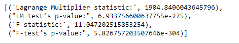
The p-value is much less than 0.05. Hence we reject the null hypothesis that the dataset is homoskedasticity. Therefore, we can say that the data has Heteroscedasticity.

Fixing Heteroscedasticity

Conclusion

This article has discussed Multicollinearity and Heteroscedasticity with their cause, detection, and handling. Now let’s summarize the article with the following key takeaways:

• Two highly correlated independent variables create Multicollinearity.
• Multicollinearity affects the model interpretability but not the model performance.
• Multicollinearity hides the individual effect of independent variables.
• Multicollinearity may occur due to wrong observation, poor experiment, dummy variable trap, and creating redundant features.
• We can fix Multicollinearity by creating new features and dropping the columns or directly removing the highly correlated features.
• Heteroscedasticity is caused due to the outliers in the dataset.
• The cone or fan-shaped scatter plot is the sign of heteroscedasticity in the dataset.

The media shown in this article is not owned by Analytics Vidhya and is used at the Author’s discretion.