This article was published as a part of the Data Science Blogathon.
In this article, we will train a classification model which uses the feature extraction + classification principle, i.e., firstly, we extract relevant features from an image and then use these feature vectors in machine learning classifiers to perform the final classification.
We will extract features from a pre-trained ResNet model. Then by using those extracted features, we will train a multiclass SVM Classifier on the STL-10 dataset and find the accuracy and Confusion matrix on the dataset and ROC Curve.
What is Resnet-50?
A convolutional neural network with 50 layers is called ResNet-50. The ImageNet database contains a pre-trained version of the network that has been trained on more than a million photos. The pretrained network can categorize images into 1000 different item categories, including several animals, a keyboard, a mouse, and a pencil.

You can download the complete .ipynb code file used in this article from here. The code is well commented on, so you can easily understand it.
In this section, we will discuss some basic Information about the dataset:
1. The STL-10 dataset is an image recognition dataset that may be used to develop algorithms for unsupervised feature learning, deep learning, and self-taught learning.
2. There are ten classes in total: – an aeroplane, a bird, a car, a cat, a deer, a dog, a horse, a monkey, a ship, and a truck.
class_present =
['airplane','bird','car','cat','deer','dog','horse','monkey',
'ship','truck']
3. The images are 96×96 pixels in size and colour.
4. Each class has 500 training photos (10 pre-defined folds) and 800 test images.
5. Unsupervised learning with 100000 unlabeled images. These samples are drawn from a larger pool of photographs with a similar look. In addition to the animals and vehicles in the designated set, it has various animals (bears, rabbits, etc.) and vehicles (trains, buses, etc.).
6. Images were gathered from ImageNet’s tagged examples.
In the form of Code, we have to do the same using the below code snippets:
from torchvision.datasets import STL10

trainset, testset = STL10('/content',transform=transform, download = True), STL10('/content',"test",transform=transform)
This section will discuss the complete machine learning pipeline to classify different classes of STL-10 datasets.
Steps to extract the features from the pre-trained ResNet model:
1. The ImageNet classification dataset is used to train the ResNet50 model.
2. The PyTorch framework is used to download the ResNet50 pretrained model.
3. The features retrieved from the last fully connected layer are used to train a multiclass SVM classifier.
4. A data loader is used to load the training and testing datasets.
5. The model and the loaded data are used to extract features.
6. The features have been visualized.
7. Every image from the training and testing sets is fed into the forward, and each embedding is saved.
8. The stored photos are fed into the pre-trained resnet50, and the weights are frozen using i.requires grad = False.
9. We load the model after that.
10. The train and test loaders are scaled using standard scalers. These two datasets are then appended to each other independently.
Data Visualization:
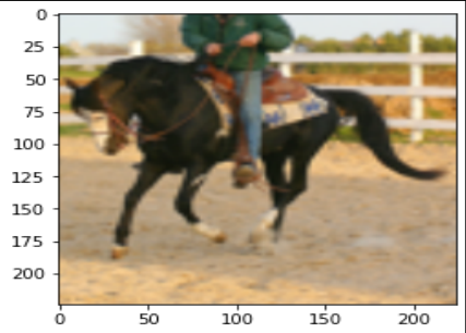
Printing one of the images from our dataset to visualize what kind of images we have on our hand to apply those algorithms:
Grid Search CV:
We will apply Grid Search CV to find the best value of hyperparameters (C, Gamma, and Kernel)
We can apply the Grid search Cross-validation technique by defining parameters in a single list and then training the same SVM model defined in sklearn with the help of those parameters to achieve the maximum performance from our model.
import numpy as np

from sklearn.model_selection import GridSearchCV

from sklearn.svm import SVC


l1 = [0.1, 1, 10, 100]

l2 = [1, 0.1, 0.01, 0.001]

l3 = ['poly']

# defining parameter range

param_grid = {'C': l1,

'gamma': l2,

'kernel': l3}


# apply grid search cross validation for finding the best set of parameters

three = 3

grid = GridSearchCV(SVC(), param_grid, refit = True, verbose = three)

grid.fit(X_trainv2, y_train)
After running the above Code, the parameters on which I have trained our model are given below:
clf2 = SVC(kernel='poly', C=C_param, gamma=gamma_param, probability=True).fit(X_trainv2,y_train)
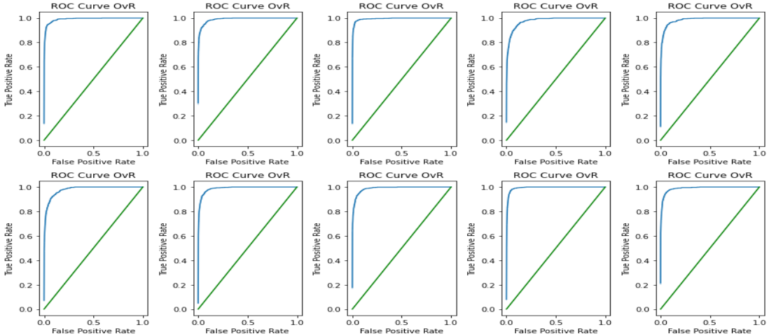
ROC Curve:
Here, we have to print the ROC curve for one of the classes versus all other classes means we are using the One versus Rest strategy, and then compare those curves with the baseline model, which means the line which is passing through the origin and making a slope of 45 with both the x and y-axis.
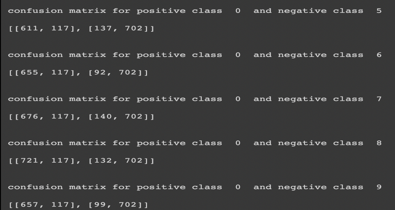
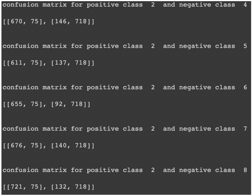
Confusion matrix:
I have attached some confusion matrices for class 0 versus all the classes where I consider 0 classes as positive and all others as unfavorable. But for other classes, I have implemented it in coding, but just for result showing, I have presented for only one of the classes.
For class 0:
For class 2:
For class 1:
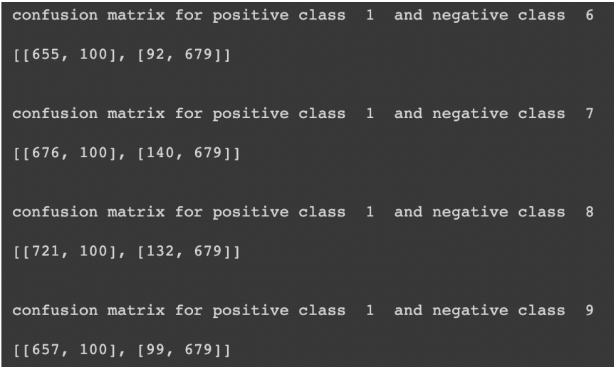
etc.
These confusion matrices show the number of false positives, false negatives, true positives, and true negatives. We can find overall and class-wise accuracy from all these values and compare the results.
Overall accuracy achieved: 76.229%
Fine-tune the ResNet 50:
We start with a default model that hasn’t been fine-tuned and look at its layer. Then there was selective fine-tuning for a single layer. Only the weights of the passed layer will be modified in this process, while we will freeze the remaining layers. We can do it on a pre-trained model, and its parameters are only updated if the layer name in the function matches the one we want to fine-tune, in which case the param requires grad is actual.
We can do any of the two types of tuning for tweaking our model:
1. Single layer tuning
2. Multi-layer tuning
The loss for training and testing is the least after fine tweaking the downsampling sub-layer, and the accuracy after fine-tuning the downsampling sub-layer in both training and testing is higher than the other sub-layers fine-tuning.
In highly deep CNNs, the vanishing gradient issue can be solved by ResNet. They operate by omitting some layers based on the presumption that intense networks shouldn’t have a more significant training error than their shallower equivalents.
ResNet has shown to be effective in various applications, but one significant downside is that deeper networks typically take weeks to train, rendering them almost unusable for practical applications.
Major points of this article:
1. Firstly, we have discussed the Resnet-50 architecture, how it works, and its pros and cons.
2. Then, we discussed the STL-10 dataset we are using in this tutorial, like the no. of images, no. of distinct classes, and image size. Etc.
3. Then, we trained the Resnet-50 model and applied feature extraction.
4. After extracting features, we implemented Grid Search CV to get the best hyperparameters.
5. Finally, discussing the Accuracy and ROC-AUC curves, we have concluded the article.
It is all for today. I hope you have enjoyed the article. If you have any doubts or suggestions, feel free to comment below. Or you can also connect with me on LinkedIn. I will be delighted to get associated with you.
Do check my other articles also.
Thanks for reading, 😊
The media shown in this article is not owned by Analytics Vidhya and is used at the Author’s discretion.
Lorem ipsum dolor sit amet, consectetur adipiscing elit,


