This article was published as a part of the Data Science Blogathon.
Introduction
In this article, we will be predicting the famous machine learning problem statement, i.e. Titanic Survival Prediction, using PySpark’s MLIB. This is one of the best datasets to get started with new concepts as we being machine learning enthusiasts, already are well aware of this particular dataset, and we are gonna do everything from scratch, i.e., from data preprocessing steps, dealing with categorical variables (converting them) and building and evaluating the model using MLIB.

The Mandatory Process to Follow
As discussed in the introduction section, we will be predicting which passenger survived the Titanic ship crash, and for that, we will be using PySpark’s MILB library. For doing so, we need first to set up an environment to start the Spark Session, and this will enable us to use all the required libraries we need for the prediction.
from pyspark.sql import SparkSession

spark = SparkSession.builder.appName('Titanic_project').getOrCreate()
spark
Code breakdown:
- The first step has to be to import the SparkSession object, and we are importing it from the pyspark.sql library.
- Then comes the part of building and creating the Spark Session; for that builder, the function is used to build it. Then for creating the same, we have the getOrCreate() method.
- To view the kind of GUI version of the session, we can simply use the object name, and it will show all the relevant information about the same, like version, app name, and Master location.
Reading the dataset in PySpark
So by far, we have set up our Spark Session. Now it’s time to read the legendary Titanic dataset, and for that, we will be using the read.csv method of PySpark, but before heading towards the coding part, let’s first look at the features that the dataset holds.
- Passenger: This is just the unique ID assigned to each passenger.
- Survived: This is the target column that our model will predict.
- P-class: This column holds the different classes of passengers who were traveling.
- Name Name of the passenger.
- Sex: Gender of the passenger.
- Age: Age of the passenger.
- SibSp: No. of Siblings and Spouse of the passenger.
- Parch Parents and no. of children of the passenger.
- Ticket: The unique number assigned to the ticket.
- Fare: Fare of the titanic ticket based on the different criteria like which class and facilities they will get.
- Cabin: Cabin number assigned to each passenger.
- Embarked: Which port will the passenger be embarked on?
data = spark.read.csv('titanic.csv',inferSchema=True,header=True)
Inference: By far, we are well aware of the fact that read.csv will read the dataset, but here we will discuss the parameters of this method
- inferSchema: Notice that this param is set to True, which means it will return the real data type of each column that our original data have; hence keeping it True is a good practice to see the real face of the dataset.
- Header: Keeping this parameter True will let the first row of the dataset as the header of the DataFrame otherwise, the original heading will also be treated as the records.
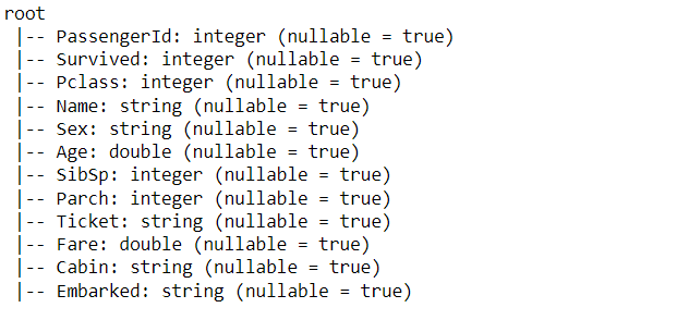
Inference: Okay! So now, from the above output, we got the original data type of each column and the information that the particular column will be able to hold the NULL value. Apart from these inferences, we should notice that features like Sex, and Embarked are in the string format, so we need to change them in categorical features.
data.columns
Output:
['PassengerId',
 'Survived',
 'Pclass',
 'Name',
 'Sex',
 'Age',
 'SibSp',
 'Parch',
 'Ticket',
 'Fare',
 'Cabin',
 'Embarked']
Inference: If one needs to find out what columns are present in the dataset, then he/she can use the columns object corresponding to the dataset.
my_cols = data.select(['Survived',
 'Pclass',
 'Sex',
 'Age',
 'SibSp',
 'Parch',
 'Fare',
 'Embarked'])
Inference: In the previous DataFrame, we got everything (the target column as well, which is not required); hence here, we are filtering the columns to only have features (dependent variables) using the select statement.
Dropping NULL values
There are various methods to deal with null values. We can either impute it with central tendency methods like mean/median/mode depending on the nature of the data, or we can simply drop all the null values here we are dropping all of them as we don’t have many of them; hence it is the better option to get rid of all at once.
Note: NA. drop() method is used to drop all the NA values from the features DataFrame, and then we assign it to a new variable which would be the final data.
my_final_data = my_cols.na.drop()
Dealing with Categorical Columns
As we discussed dealing with the categorical columns which are now in the String state, but as we know, String type is not accepted by any ML algorithm, so we need to deal with it, and for that, we have to go through a set of operations/steps in PySpark.
So, let’s break down each step and convert the necessary features columns.
Vector Assembler and OneHotEncoder
Vector Assembler: From the name itself it is indicating that it kind of puts together columns in a collective vectorized format i.e., all the features get stacked up as a single unit in the form of a vector, and this is one of the rules as well that MLIB library takes all the features as a single unit only.
One Hot Encoder: There are multiple ways of dealing with categorical variables this time going with One hot encoder where each categorical value is separated into an independent column and gets the binary value i.e. either 0 or 1.
from pyspark.ml.feature import (VectorAssembler,VectorIndexer,
                                OneHotEncoder,StringIndexer)

gender_indexer = StringIndexer(inputCol='Sex',outputCol='SexIndex')
gender_encoder = OneHotEncoder(inputCol='SexIndex',outputCol='SexVec')

embark_indexer = StringIndexer(inputCol='Embarked',outputCol='EmbarkIndex')
embark_encoder = OneHotEncoder(inputCol='EmbarkIndex',outputCol='EmbarkVec')

assembler = VectorAssembler(inputCols=['Pclass',
 'SexVec',
 'Age',
 'SibSp',
 'Parch',
 'Fare',
 'EmbarkVec'],outputCol='features')
Code breakdown:
- As discussed, the Vector assembler and One Hot encoding technique are required for conversion; hence we imported both of them from the ml. feature library of PySpark.
- While importing other important methods, note that StringIndexer was also there, which would be responsible for converting the String type to a categorical type.
- Then One Hot Encoder will convert each categorical value to its binary value, i.e., 0 or 1, by its predefined object. Repeating the same process for the “Embarked” column as we did for the “Gender” column.
- At last, Vector Assembler will put together all the preprocessed feature columns together and remove the unwanted ones.
from pyspark.ml.classification import LogisticRegression
So we are good to go with the model development phase, and the first thing we need to import is the ML algorithm; for this particular problem statement, we have to predict the categorical data; hence classification machine learning algorithm should be accessed, i.e.,, Logistic Regression.
Pipelines from PySpark
Sometimes coping with the whole process of model development is complex. We get stuck to choosing the right flow if the execution in this type of problem Pipelines from PySpark comes in to rescue us as it helps maintain the execution cycle flow so that each step should be performed at its best given stage neither before nor soon.
from pyspark.ml import Pipeline

log_reg_titanic = LogisticRegression(featuresCol='features',labelCol='Survived')

pipeline = Pipeline(stages=[gender_indexer,embark_indexer,
                           gender_encoder,embark_encoder,
                           assembler,log_reg_titanic])

train_titanic_data, test_titanic_data = my_final_data.randomSplit([0.7,.3])

fit_model = pipeline.fit(train_titanic_data)

results = fit_model.transform(test_titanic_data)
Code breakdown:
- First and foremost Pipeline module is being accessed and imported by the pyspark. ml library.
- Then for developing the model, the Logistic Regression method is used in the parameters passing in the features columns and label (independent) column.
- Now comes the Pipeline method, where one can look in the stages section that all the preprocessed steps are lined up one after the other.
- Then using the random split() method, the final dataset is broken down into a training set of 70% and a testing set of 30%.
- At last, it’s important to have all the changes committed for that we are first fitting the pipeline with training data and transforming the testing data with the pipeline model.
Model Evaluation
Okay! So we are now in the Model Evaluation phase which means development is already done and now we should evaluate it from evaluating, we mean that it should be working as per our requirement with good results i.e., good accuracy over testing data.
from pyspark.ml.evaluation import BinaryClassificationEvaluator
my_eval = BinaryClassificationEvaluator(rawPredictionCol='prediction',
labelCol='Survived')
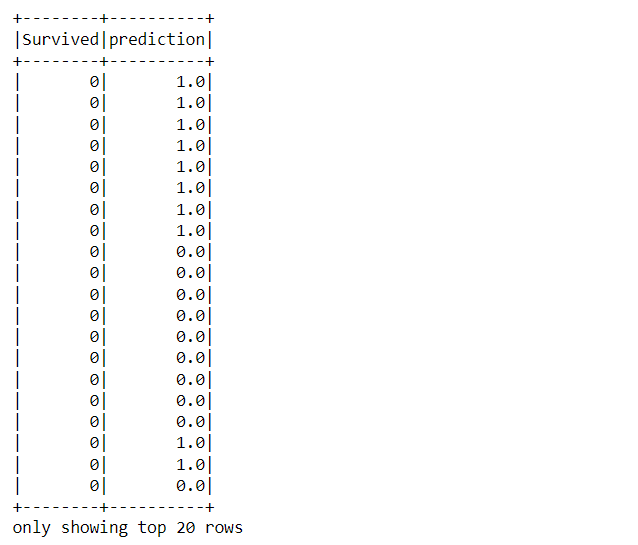
results.select('Survived','prediction').show()
Output:
Code breakdown:
- Imported the Binary Classifier as this problem statement has the binary type of target column.
- Then by applying the Binary Classification evaluator object, we are passing in the values to the raw prediction column and the label column
- At the end, when the DataFrame has both Survived and Prediction columns after the evaluation, then it is shown using a select statement.
Conclusion
Here we come in the final section of this article, where we will allow ourselves to go along with whatever we did so far in this article, i.e. from starting the spark session to building and evaluating the model, we will discuss each step in brief.
- Firstly we started the spark session and read the famous titanic survivals dataset using PySpark data preprocessing techniques.
- Then, we dealt with NULL values by dropping all of them. Along with that, we also handled the categorical features and converted them to relevant types using Vector Assembler and One Hot Encoder.
- During the next phase, we came across the concept of Pipelines which helped us to build an end-to-end pipeline of all the stages.
- At last, we build the Logistic regression model using PySpark MLIB and later evaluate it too so that we should see how well our model performed based on the testing data.
The media shown in this article is not owned by Analytics Vidhya and is used at the Author’s discretion.


