This article was published as a part of the Data Science Blogathon.
Introduction
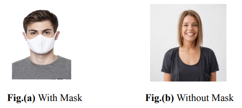
In this article, we will create a Mask v/s No Mask classifier using CNN and Machine Learning Classifiers. It will detect whether a person is wearing a face mask or not. We will learn everything from scratch, and I will explain every step. I require your basic understanding of Machine Learning and Data Science. I have implemented it on my local Windows 10 machine, but if you want, you can also implement it on Google Colab.
A Convolutional Neural network (CNN) is a type of Artificial Neural network designed to process pixel data. They are used explicitly in Image Processing and Image Recognition.
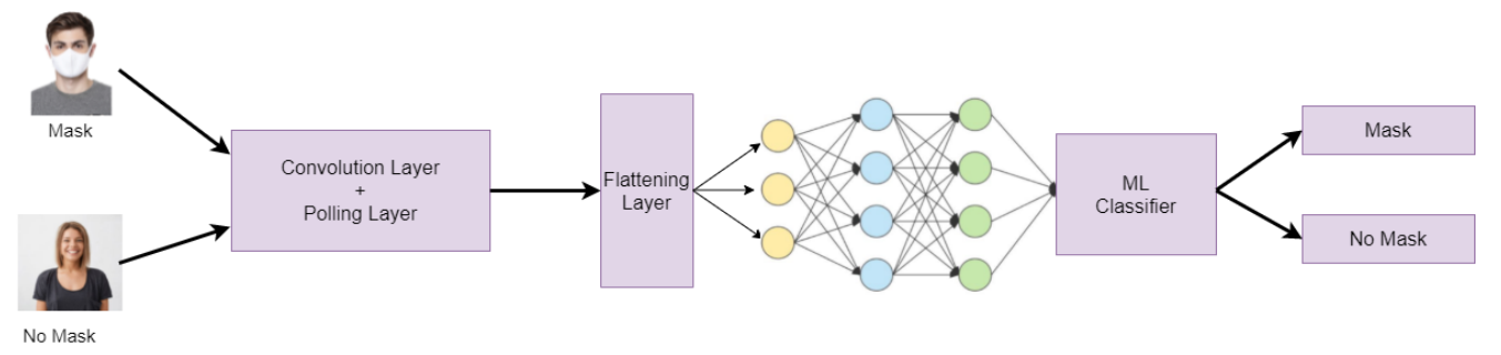
CNN Model Pipeline
First, we will input the RGB images of size 224×224 pixels. Then these images will go into a CNN model that will extract 128 relevant feature vectors from them. Then we will use these feature vectors to train our various machine learning classifiers, like Logistic Regression, Random Forest, etc., to classify whether the person in that image is wearing a mask or not. You can refer to the below diagram for a better understanding.
Let’s get started, 😉
Working of Code to Train CNN Model
In this section, we will learn about the coding part. We will discuss the loading and preprocessing of the dataset, training the CNN Model, and extracting feature vectors to train machine learning classifiers.
Importing Necessary Libraries:
We will import all the necessary libraries that we require for this project.
We will use libraries like Numpy, which is used to perform complex mathematical calculations. Pandas load and preprocess the dataset, and many more libraries are used.
import numpy as np

import pandas as pd

import matplotlib.pyplot as plt

import os

from itertools import cycle

from sklearn.model_selection import train_test_split

from tensorflow.keras.models import Model

from tensorflow.keras.layers import Dropout, Dense, AveragePooling2D, Flatten ,Dense, Input

from sklearn.metrics import classification_report, confusion_matrix

import cv2
from sklearn.metrics import roc_curve, auc

from sklearn.preprocessing import label_binarize

from scipy import interp

from sklearn.ensemble import RandomForestClassifier

from tensorflow.keras.preprocessing.image import ImageDataGenerator

from tensorflow.keras.applications import MobileNetV2

from tensorflow.keras.optimizers import Adam
Loading and Preprocessing of Dataset
You can download the dataset from that GitHub Repo.
Clone your Dataset from the above repository.
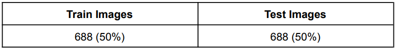
This dataset contains more than 1200+ images of different people wearing a face mask or not. After loading the dataset, we will preprocess it. It involves splitting into train and test datasets, converting pixel values between 0 to 1, and converting the labels into one-hot encoded labels.
Below is the code for loading and preprocessing the dataset. It is well commented so that you can understand it easily.
In the below code, we will first read all the images from the folder and then store them in an array by resizing them into 224×224 pixels. After that, we will label these images. Images with masks have a label 0, and images without masks have a label 1. Finally, we will split this dataset into training and testing using the sklearn function named train test split.
# List all the images with a mask from the master directory.
filenames = os.listdir("observations-master/experiements/data/with_mask")

np.random.shuffle(filenames)

print(filenames) # Read all the images from that directory and resize them into 224x224 pixels.

with_mask_data = [cv2.resize(cv2.imread("observations-master/experiements/data/with_mask/"+img), (224,224)) for img in filenames]

print(len(with_mask_data))
# The above similar step is performed for the images that don’t contain a mask.
filenames = os.listdir("observations-master/experiements/data/without_mask")

np.random.shuffle(filenames)

print(filenames)

without_mask_data = [cv2.resize(cv2.imread("observations-master/experiements/data/without_mask/"+img), (224,224)) for img in filenames]

print(len(without_mask_data))
# We have combined both arrays to make a single array, converting each pixel value between 0 and 1 by dividing them by 255.
data = np.array(with_mask_data + without_mask_data).astype('float32')/255 # Label of the image with a mask - 0 # Label of the image without mask - 1

labels = np.array([0]*len(with_mask_data) + [1]*len(without_mask_data))

print(data.shape) # Splitting the data into training and testing sets.

(training_data, testing_data, training_label, testing_label) = train_test_split(data, labels, test_size=0.50, stratify=labels, random_state=42)
print(training_data.shape) # Function to Plot the Accuracy/Loss Curves

def plot_acc_loss(result, epochs):

acc = result.history['accuracy']

loss = result.history['loss']

val_acc = result.history['val_accuracy']

val_loss = result.history['val_loss']

plt.figure(figsize=(15, 5))

plt.subplot(121)

plt.plot(range(1,epochs), acc[1:], label='Train_acc')

plt.plot(range(1,epochs), val_acc[1:], label='Val_acc')

plt.title('Accuracy over ' + str(epochs) + ' Epochs', size=15)

plt.legend()

plt.grid(True)

plt.subplot(122)

plt.plot(range(1,epochs), loss[1:], label='Train_loss')

plt.plot(range(1,epochs), val_loss[1:], label='Val_loss')

plt.title('Loss over ' + str(epochs) + ' Epochs', size=15)

plt.legend()

plt.grid(True)

plt.show()
Building The Convolutional Neural Network (CNN)
Now we will build our Convolutional Neural network. Firstly we have used an image data generator to increase the number of images in our dataset. This image generator will generate some more photos from these existing images. It performs some rotation clockwise or anti-clockwise, changing the contrast, performing zoom-in or zoom-out, etc.
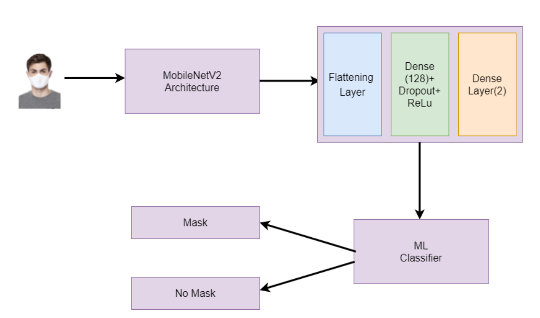
After that, we will use a pre-trained MobileNetV2 Architecture to train our model. It is a transfer learning model. Transfer learning is when pre-trained models are used to train new deep learning models, i.e. if two models perform similar tasks, we can share knowledge. After applying transfer learning, we will apply a flattening layer to convert the 2D matrix into a 1D array. After that, we will apply dense and dropout layers to perform the classification.
Finally, we will train our model by taking the batch size as 32 and the number of epochs as 25. You can take any other values according to your computational power.
Code for training the Convolutional Neural Network Model:
We will build our transfer learning MobileNetV2 Architecture, a pre-trained CNN model. Firstly, we will generate some more images from our dataset using the Image Data Generator. After that, we will set our hyperparameters like learning rate, batch size, no. of epochs, etc. And then finally, we will train our model and check its accuracy on the test set.
# Image data generator to generate more images.

generator = ImageDataGenerator(

rotation_range=20,

zoom_range=0.15,

width_shift_range=0.2,

height_shift_range=0.2,

shear_range=0.15,

horizontal_flip=True,

fill_mode="nearest")
# Setting the hyperparameters.
learning_rate = 0.0001

epoch = 25

batch_size = 32

# Training the mobile net v2 architecture.
transfer_learning_model = MobileNetV2(weights="imagenet", include_top=False,

input_tensor=Input(shape=(224, 224, 3)))


model_main = transfer_learning_model.output

model_main = AveragePooling2D(pool_size=(7, 7))(model_main) # Applying the flattening layer.

model_main = Flatten(name="flatten")(model_main)

model_main = Dense(128, activation="relu", name="dense_layer")(model_main)

model_main = Dropout(0.5)(model_main)

model_main = Dense(2, activation="softmax")(model_main)

cnn = Model(inputs=transfer_learning_model.input, outputs=model_main)

for row in transfer_learning_model.layers:

row.trainable = False


optimizer = Adam(lr=learning_rate, decay=learning_rate / epoch)

cnn.compile(loss="sparse_categorical_crossentropy", optimizer=optimizer,

metrics=["accuracy"])

# Train the CNN model

history = cnn.fit(

generator.flow(training_data, training_label, batch_size=batch_size),

steps_per_epoch=len(training_data) // batch_size,

validation_data=(testing_data, testing_label),

validation_steps=len(testing_data) // batch_size,

epochs=epoch)


Evaluate the trained model
# Evaluate the model on the test set.

cnn.evaluate(testing_data, testing_label)

plot_acc_loss(history, 25)
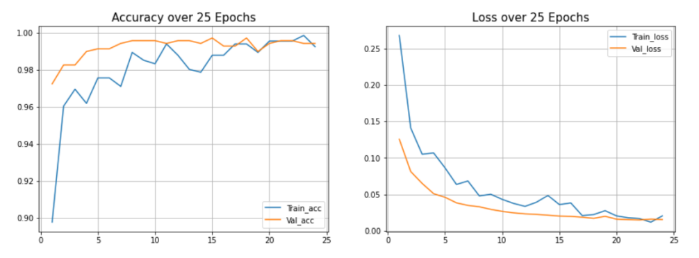
We Obtained An Accuracy of 99.42% on the Test Set
Using Machine Learning Classifiers
Now, we will extract 128 Relevant Feature Vectors from our previously trained CNN Model & applying them to different ML Classifiers. We will use the following Machine Learning Classifiers:
Xtreme Gradient Boosting:
Extreme Gradient Boosting (XGBoost) is an open-source library that efficiently and effectively implements the gradient boosting algorithm. First, import necessary libraries and then define the classifier as XGBClassifier. After fitting it, represent predictions and accuracy scores. We get accuracy, confusion matrix, and classification report as output. Here, we got 98.98% of our accuracy.
Random Forest Classifier:
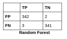
Random Forest is a classifier that contains several decision trees on various subsets of the given dataset and takes the average to improve the predictive accuracy of that dataset. The more significant number of trees in the forest leads to higher accuracy and prevents the problem of overfitting. First, import necessary libraries and then define the classifier as RandomForestClassifier. After fitting it, represent predictions and accuracy scores. We get accuracy, confusion matrix, and classification report as output. Here, we got 99.41% as our accuracy, which is more than XGBoost.
Logistic Regression:
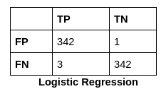
Logistic regression is a supervised learning classification algorithm used to predict the probability of a target variable. The target or dependent variable’s nature is dichotomous, meaning there would be only two possible classes. Here, we got 99.70% as our accuracy, which is more than XGBoost but slightly less than random forest.
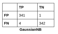
Gaussian distribution:
A probability distribution symmetric around the mean is the normal distribution, sometimes called the Gaussian distribution. It demonstrates that data close to the mean occur more frequently than data far from the mean. The bell curve represents the normal distribution on a graph.
Below is the code for extracting the essential feature vectors and putting these feature vectors in Machine Learning Classifiers.
After training our CNN model, we will now apply feature extraction and extract 128 relevant feature vectors from these images. And these appropriate feature vectors are fed into our various machine-learning classifiers to perform the final classification.
We have used various machine learning models like XGBoost, Random Forest, Logistic Regression, GaussianNB, etc. We will select the model which gives us the best accuracy.
from keras.models import Model

layer_name='dense_layer' # Extracting the layer from the above CNN model, which contains 128neurons.

new_model = Model(inputs=cnn.input,

outputs=cnn.get_layer(layer_name).output)


new_model.summary()

# Get new training data that only contains these 128 features.

training_image_features = new_model.predict(training_data)

training_image_features = pd.DataFrame(data=training_image_features)


testing_image_features = new_model.predict(testing_data)

testing_image_features = pd.DataFrame(data=testing_image_features)


# Perform the classification using XGBoost Classifier. from xgboost import XGBClassifier

from sklearn.metrics import accuracy_score

classifier = XGBClassifier()

classifier.fit(training_image_features, training_label)

predictions = classifier.predict(testing_image_features) # Getting the accuracy score

accuracy = accuracy_score(predictions, testing_label)

print(f'{accuracy*100}%') # Getting the confusion matrix.

cf = confusion_matrix(predictions, testing_label)

print(cf)

from sklearn.metrics import classification_report

c_r = classification_report(predictions, testing_label, output_dict=True)

print(c_r)

# Perform the classification using RandomForest Classifier.

from sklearn.ensemble import RandomForestClassifier

rfc = RandomForestClassifier()

rfc.fit(training_image_features, training_label)

prediction = rfc.predict(testing_image_features)

accuracy = accuracy_score(prediction, testing_label)

print(f'{accuracy*100}%')

cf = confusion_matrix(prediction, testing_label)

print(cf)

from sklearn.metrics import classification_report

c_r = classification_report(prediction, testing_label, output_dict=True)

print(c_r)

# Perform the classification using LogisticRegression

from sklearn.linear_model import LogisticRegression

lin_r = LogisticRegression()

lin_r.fit(training_image_features, training_label)

prediction = lin_r.predict(testing_image_features)

accuracy = accuracy_score(prediction, testing_label)

print(f'{accuracy*100}%')

cf = confusion_matrix(prediction, testing_label)

print(cf)

from sklearn.metrics import classification_report

c_r = classification_report(prediction, testing_label, output_dict=True)

print(c_r)

# Perform the classification using GaussianNB

from sklearn.naive_bayes import GaussianNB

n_b = GaussianNB()

n_b.fit(training_image_features, training_label)

prediction = n_b.predict(testing_image_features)

accuracy = accuracy_score(prediction, testing_label)

print(f'{accuracy*100}%')

cf = confusion_matrix(prediction, testing_label)

print(cf)

from sklearn.metrics import classification_report

c_r = classification_report(prediction, testing_label, output_dict=True)

print(c_r)
Results
In this section, we will discuss the results of our classification. We will discuss how much accuracy we have achieved and what is the precision, recall and f1-score. If you want to learn more about these performance scores, there is a lovely article to which you can refer.
Accuracy: One parameter for assessing classification models is accuracy. The percentage of predictions that our model correctly predicted is known as accuracy. The following is the official definition of accuracy: The number of accurate guesses equals the accuracy amount of guesses overall.
Precision: Precision is calculated by dividing the total number of positive predictions by the proportion of genuine positives (i.e., the number of true positives plus the number of false positives).
F1 Score: One of the most crucial assessment measures in machine learning is the F1 score. Combining accuracy and recall, two measures that would typically be in competition, it elegantly summarises the prediction ability of a model.
Below are the performance scores of all the machine learning classifiers we used to train our model. Logistic Regression gives the highest accuracy, which is 99.709%.

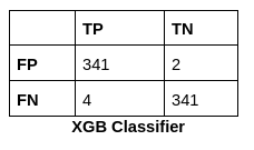
The confusion matrix for all the Machine Learning Classifiers are:
The Confusion Matrix is an NxN matrix that summarises the predicted results. It contains the number of correct and incorrect predictions broken by each class.
Complete Code
In this section, I have shared the complete code used in this project. In addition to the above code, this code also contains the code to plot the ROC-AUC curves of your machine-learning model.
A ROC curve (receiver operating characteristic curve) is a graph showing the performance of a classification model at all classification thresholds. This curve plots two parameters: True Positive Rate. False Positive Rate.
Firstly we loaded the dataset. Then we read the images using the OpenCV library and store them in an array by converting them into 224×224 pixel sizes. After that, we have to make labels for both classes, i.e., mask and no mask. Then we discussed the code for Image Data Generator and MobileNetV2 Architecture. Further, we have trained our CNN model after setting the hyperparameters like epochs, batch size, etc. And after the completion of 25 epochs, we got an accuracy of 99.42% on the test set.
After training the CNN model, we applied feature extraction and extracted 128 feature vectors from the dense layer and applied these feature vectors to the machine learning model to get the final classification. Then we have written the code for evaluating various performance matrices like Accuracy Score, F1-Score, Precision, etc. Finally, we plotted the ROC-AUC curve for the best-performing machine learning model.
import numpy as np

import pandas as pd

import matplotlib.pyplot as plt

import os

from itertools import cycle

from sklearn.model_selection import train_test_split

from tensorflow.keras.models import Model

from tensorflow.keras.layers import Dropout, Dense, AveragePooling2D, Flatten ,Dense, Input

from sklearn.metrics import classification_report, confusion_matrix

import cv2


from sklearn.metrics import roc_curve, auc

from sklearn.preprocessing import label_binarize

from scipy import interp

from sklearn.ensemble import RandomForestClassifier

from tensorflow.keras.preprocessing.image import ImageDataGenerator

from tensorflow.keras.applications import MobileNetV2

from tensorflow.keras.optimizers import Adam


def plot_acc_loss(result, epochs):

acc = result.history['accuracy']

loss = result.history['loss']

val_acc = result.history['val_accuracy']

val_loss = result.history['val_loss']

plt.figure(figsize=(15, 5))

plt.subplot(121)

plt.plot(range(1,epochs), acc[1:], label='Train_acc')

plt.plot(range(1,epochs), val_acc[1:], label='Val_acc')

plt.title('Accuracy over ' + str(epochs) + ' Epochs', size=15)

plt.legend()

plt.grid(True)

plt.subplot(122)

plt.plot(range(1,epochs), loss[1:], label='Train_loss')

plt.plot(range(1,epochs), val_loss[1:], label='Val_loss')

plt.title('Loss over ' + str(epochs) + ' Epochs', size=15)

plt.legend()

plt.grid(True)

plt.show()


# filenames = glob(mypath +'with_mask/'+'*.jpg')

filenames = os.listdir("observations-master/experiements/data/with_mask")

np.random.shuffle(filenames)

print(filenames) # 460 , 116

with_mask_data = [cv2.resize(cv2.imread("observations-master/experiements/data/with_mask/"+img), (224,224)) for img in filenames]

print(len(with_mask_data))


filenames = os.listdir("observations-master/experiements/data/without_mask")

np.random.shuffle(filenames)

print(filenames) # 460 , 116

without_mask_data = [cv2.resize(cv2.imread("observations-master/experiements/data/without_mask/"+img), (224,224)) for img in filenames]

print(len(without_mask_data))


data = np.array(with_mask_data + without_mask_data).astype('float32')/255

labels = np.array([0]*len(with_mask_data) + [1]*len(without_mask_data))

print(data.shape)

(training_data, testing_data, training_label, testing_label) = train_test_split(data, labels, test_size=0.50, stratify=labels, random_state=42)

print(training_data.shape)


generator = ImageDataGenerator(

rotation_range=20,

zoom_range=0.15,

width_shift_range=0.2,

height_shift_range=0.2,

shear_range=0.15,

horizontal_flip=True,

fill_mode="nearest")


learning_rate = 0.0001

epoch = 25

batch_size = 32


transfer_learning_model = MobileNetV2(weights="imagenet", include_top=False,

input_tensor=Input(shape=(224, 224, 3)))


model_main = transfer_learning_model.output

model_main = AveragePooling2D(pool_size=(7, 7))(model_main)

model_main = Flatten(name="flatten")(model_main)

model_main = Dense(128, activation="relu", name="dense_layer")(model_main)

model_main = Dropout(0.5)(model_main)

model_main = Dense(2, activation="softmax")(model_main)

cnn = Model(inputs=transfer_learning_model.input, outputs=model_main)

for row in transfer_learning_model.layers:

row.trainable = False


optimizer = Adam(lr=learning_rate, decay=learning_rate / epoch)

cnn.compile(loss="sparse_categorical_crossentropy", optimizer=optimizer,

metrics=["accuracy"])


history = cnn.fit(

generator.flow(training_data, training_label, batch_size=batch_size),

steps_per_epoch=len(training_data) // batch_size,

validation_data=(testing_data, testing_label),

validation_steps=len(testing_data) // batch_size,

epochs=epoch)


cnn.evaluate(testing_data, testing_label)


plot_acc_loss(history, 25)


from keras.models import Model

layer_name='dense_layer'

new_model = Model(inputs=cnn.input,

outputs=cnn.get_layer(layer_name).output)


new_model.summary()


training_image_features = new_model.predict(training_data)

training_image_features = pd.DataFrame(data=training_image_features)


testing_image_features = new_model.predict(testing_data)

testing_image_features = pd.DataFrame(data=testing_image_features)


from xgboost import XGBClassifier


from sklearn.metrics import accuracy_score

classifier = XGBClassifier()

classifier.fit(training_image_features, training_label)

predictions = classifier.predict(testing_image_features)

accuracy = accuracy_score(predictions, testing_label)

print(f'{accuracy*100}%')

cf = confusion_matrix(predictions, testing_label)

print(cf)

from sklearn.metrics import classification_report

c_r = classification_report(predictions, testing_label, output_dict=True)

print(c_r)


from sklearn.ensemble import RandomForestClassifier

rfc = RandomForestClassifier()

rfc.fit(training_image_features, training_label)

prediction = rfc.predict(testing_image_features)

accuracy = accuracy_score(prediction, testing_label)

print(f'{accuracy*100}%')

cf = confusion_matrix(prediction, testing_label)

print(cf)

from sklearn.metrics import classification_report

c_r = classification_report(prediction, testing_label, output_dict=True)

print(c_r)


from sklearn.linear_model import LogisticRegression

lin_r = LogisticRegression()

lin_r.fit(training_image_features, training_label)

prediction = lin_r.predict(testing_image_features)

accuracy = accuracy_score(prediction, testing_label)

print(f'{accuracy*100}%')

cf = confusion_matrix(prediction, testing_label)

print(cf)

from sklearn.metrics import classification_report

c_r = classification_report(prediction, testing_label, output_dict=True)

print(c_r)


from sklearn.naive_bayes import GaussianNB

n_b = GaussianNB()

n_b.fit(training_image_features, training_label)

prediction = n_b.predict(testing_image_features)

accuracy = accuracy_score(prediction, testing_label)

print(f'{accuracy*100}%')

cf = confusion_matrix(prediction, testing_label)

print(cf)

from sklearn.metrics import classification_report

c_r = classification_report(prediction, testing_label, output_dict=True)

print(c_r)


# Binarize the output

y = label_binarize(training_label, classes=[0, 1])

y_test = label_binarize(testing_label, classes=[0, 1])

n_classes = 2


# Learn to predict each class against the other

classifier = RandomForestClassifier()

classifier.fit(training_image_features, y)

y_score = classifier.predict(testing_image_features)


print(accuracy_score(y_score, y_test))


# Compute the ROC curve and ROC area for each class

fpr = dict()

tpr = dict()

roc_auc = dict()

for i in range(n_classes):

fpr[i], tpr[i], _ = roc_curve(y_test[:, i], y_score[:, i])

roc_auc[i] = auc(fpr[i], tpr[i])


# Compute micro-average ROC curve and ROC area

fpr["micro"], tpr["micro"], _ = roc_curve(y_test.ravel(), y_score.ravel())

roc_auc["micro"] = auc(fpr["micro"], tpr["micro"])


# First aggregate all false positive rates

all_fpr = np.unique(np.concatenate([fpr[i] for i in range(n_classes)]))


# Then interpolate all ROC curves at these points

mean_tpr = np.zeros_like(all_fpr)

for i in range(n_classes):

mean_tpr += interp(all_fpr, fpr[i], tpr[i])


# Finally, average it and compute AUC

mean_tpr /= n_classes


fpr["macro"] = all_fpr

tpr["macro"] = mean_tpr

roc_auc["macro"] = auc(fpr["macro"], tpr["macro"])


# Plot all ROC curves

plt.figure()

plt.plot(fpr["micro"], tpr["micro"],

label='micro-average ROC curve (area = {0:0.2f})'

''.format(roc_auc["micro"]),

color='deeppink', linestyle=':', linewidth=4)


plt.plot(fpr["macro"], tpr["macro"],

label='macro-average ROC curve (area = {0:0.2f})'

''.format(roc_auc["macro"]),

color='navy', linestyle=':', linewidth=4)


colors = cycle(['aqua', 'darkorange', 'cornflowerblue'])

for i, color in zip(range(n_classes), colors):

plt.plot(fpr[i], tpr[i], color=color,

label='ROC curve of class {0} (area = {1:0.2f})'

''.format(i, roc_auc[i]))


plt.plot([0, 1], [0, 1], 'k--')

plt.xlim([0.0, 1.0])

plt.ylim([0.0, 1.05])

plt.xlabel('False Positive Rate')

plt.ylabel('True Positive Rate')

plt.title('Some extension of Receiver operating characteristic to multi-class')

plt.legend(loc="lower right")

plt.show()
Experimental Setups Used:
We have implemented the proposed classification system for classification using Python 3.8 programming language with a processor of IntelR Core i5-1155G7 CPU @ 2.30GHz × 8 and RAM of 8GB running on Windows 10 with NVIDIA Geforce MX 350 with 2GB Graphics.
Conclusion
In this work, we have presented the use of Convolutional Networks and Machine Learning classifiers to classify Mask And No Mask effectively. We also used image augmentation in our dataset to normalise the images. After Image Feature extraction through CNN, machine learning algorithms are applied for final classification leading to the best result obtained by Convolutional Neural Networks with an accuracy of 99.42% and 99.21% for Random Forest and 99.70% for Logistic Regression, which is the Highest Among All. Therefore, this approach to images and Image Processing Techniques can be a massive, faster, and cost-effective way of classification. Training with more massive datasets and testing in the field with a larger cohort can improve accuracy.
Key takeaways of this article:
1. We have discussed the CNN and Machine Learning Classifiers.
2. Then, we jumped on the coding part and discussed loading and preprocessing the dataset.
3. Further, we have trained the CNN model and then discussed the test and validation accuracy.
4. After that, we extracted the feature vectors and put them in the machine learning classifiers.
5. Finally, we have concluded this article.
It is all for today. I hope you have enjoyed the article. If you have any doubts or suggestions, feel free to comment below. Or you can also connect with me on LinkedIn. I will be delighted to get associated with you.
Do check my other articles also.
Thanks for reading, 😊
The media shown in this article is not owned by Analytics Vidhya and is used at the Author’s discretion.
I am currently pursuing my Bachelor of Technology (B.Tech.) in Electrical Engineering and Engineering from the Indian Institute of Technology Jodhpur(IITJ). I am very enthusiastic about Machine learning, and Software Development. Feel free to connect with me on Linkedin.


A lot have been learnt on the CNN models