Ever wondered how the text suggestions are automatically generated when you start googling? If you have, you are at the right place to explore it. Any guesses how? Yes, you got it! It’s the beauty of Natural Language Processing’s Transformers. In this article, you will get all about the BERT Architecture,its needs and Input and output of BERT.
Table of contents
A Quick Recap of Transformers in NLP
A transformer has rapidly become the dominant architecture for NLP surpassing alternative neural models such as CNN, RNN, and LSTM in performance for tasks in both natural language understanding and natural language generation. Let’s have a quick look at transformers.
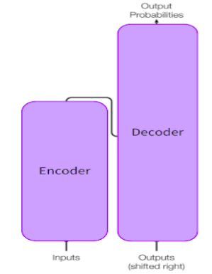
Transformers are used to learn the long-range dependencies between words in a sentence while performing sequence-to-sequence modeling. Transformers achieved work better than other models by solving the cons like variable-length input, parallelization, vanishing or exploding gradients, the massive size of data, etc. It uses an attention mechanism that is part of a neural architecture that enables it to dynamically highlight relevant features of the input data, focusing only on the necessary features/words. Let’s look at an example:
- “I poured water from the bottle into the cup until it was full.”
- It here refers to a cup
- “I poured water from the bottle into the cup until it was empty.”
- It here refers to a bottle
One single replacement in the sentence changed the reference of the object “it”. It’s easy for me or you to identify the subject/object that “it” refers to, but the ultimate task is to make a machine learn this. So If we are translating such a sentence or trying to generate text, the machine must know the word “it” refers to. This can be achieved via the deep learning mechanism “attention”. The use of an attention mechanism gives transformers high potential. One such application of transformer is BERT. Let’s dive deeper into BERT.
An Overview of BERT Architecture
BERT stands for Bidirectional Encoder Representations from Transformers(BERT) and is used to efficiently represent highly unstructured text data in vectors. BERT is a trained Transformer Encoder stack. Primarily it has two model sizes: BERT BASE and BERT LARGE.
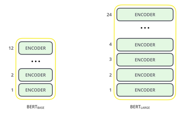
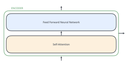
The figure above clearly shows the difference between BERTBASE and BERTLARGE. i.e, the total number of encoders. The following figure describes the design of a single encoder.
BERTBASE (L=12, H=768, A=12, Total Parameters=110M)
BERTLARGE (L=24, H=1024, A=16, Total Parameters=340M)
Where L = Number of layers (i.e; the total number of encoders)
H = Hidden size
A = Number of self-attention heads
BERT Model Input
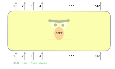
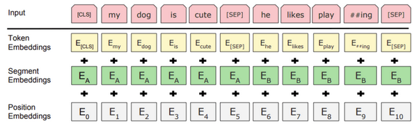
The input representation could be a single sentence or a pair of sentences. Before passing the input into BERT, a few special tokens need to be embedded.
[CLS] – The first token of every sequence(refers to the input token sequence to BERT) is always a special classification token.
[SEP] – Sentence pairs are packed together into a single sequence. We can differentiate the sentences via this special token. (The other way to differentiate is by adding a learned embedding to every token, indicating whether it belongs to sentence A or sentence B)
The input representation of a given token(word) is constructed by summing the corresponding token, segment, and position embeddings.
Once the input tokens are ready, they keep flowing up the stack. Each layer applies self-attention, passes its results through a feed-forward network, and then hands it off to the next encoder. In terms of architecture, this remains identical to the Transformer up until this point. It’s at the output that we first start seeing how things diverge. With advancements like BERT language model, sentence prediction, pre-trained BERT models, natural language processing (NLP), next sentence prediction, masked language model, NLP tasks, masked language modeling, sentiment analysis, and human language, the capabilities and applications of such models expand significantly.
BERT Model Output
Each position outputs a vector of size H. Now, this output can be used as input for the tasks to be performed, for example, classification, text generation, etc.
Why do we Need BERT?
Why do we need BERT when we have word embeddings?
A word can have different meanings in different contexts. For example, “I encountered a bat when I went to buy a cricket bat.” Here, the first occurrence of the word bat refers to a mammal, and the second refers to a playing bat. In such cases, the first and second occurrence of the word bat needs to be represented differently as they mean different, but word embeddings treat it as the same word. Hence, a single representation of the word bat will be generated. This will lead to incorrect predictions. The BERT embedding will be able to distinguish and capture the two different semantic meanings by producing two different vectors for the same word, “bat.”
Sentiment Analysis Using BERT and Hugging Face
Problem Statement:
Analyzing sentiments of the tweets on the first 2016 GOP Presidential Debate.
- Installing the Hugging Face’s Transformers Library
Hugging Face is one of the most popular Natural Language Processing communities for deep learning researchers, hands-on practitioners, and educators. Transformers library (formerly known as PyTorch-transformers) provides a wide range of general-purpose architectures (BERT, GPT-2, RoBERTa, XLM, DistilBert, etc.) for Natural Language Understanding (NLU) and Natural Language Generation (NLG) with a wide range of pre-trained models
!pip install transformers- Loading & Understanding BERT
2.1 Download Pretrained BERT model
We will use the uncased pre-trained version of the BERT base model. It was trained on lower-cased English text.
from transformers import BertModel
bert = BertModel.from_pretrained('bert-base-uncased')
2.2 Tokenization and Input Formatting
Download BERT Tokenizer
from transformers import BertTokenizerFast
tokenizer = BertTokenizerFast.from_pretrained('bert-base-uncased', do_lower_case=True)
Steps Followed for Input Formatting
- Tokenization
- Special Tokens
Prepend the [CLS] token to the start of the sequence.
Append the [SEP] token to the end of the sequence. - Pad sequences
- Converting tokens to integers
- Create Attention masks to avoid pad tokens
#input text
text = "Jim Henson was a puppeteer"
sent_id = tokenizer.encode(text,
                           # add [CLS] and [SEP] tokens
                           add_special_tokens=True,
                           # specify maximum length for the sequences
                           max_length = 10,
                           truncation = True,
                           # add pad tokens to the right side of the sequence
                           pad_to_max_length='right')
# print integer sequence
print("Integer Sequence: {}".format(sent_id))
# convert integers back to text
print("Tokenized Text:",tokenizer.convert_ids_to_tokens(sent_id))
Output
Integer Sequence: [101, 3958, 27227, 2001, 1037, 13997, 11510, 102, 0, 0]
Tokenized Text: ['[CLS]', 'jim', 'henson', 'was', 'a', 'puppet', '##eer', '[SEP]', '[PAD]', '[PAD]']
Decode the tokenized text
decoded = tokenizer.decode(sent_id)
print("Decoded String: {}".format(decoded))
Output
Decoded String: [CLS] jim henson was a puppeteer [SEP] [PAD] [PAD]
Mask to avoid performing attention to padding token indices.
Mask values: 1 for tokens NOT MASKED, 0 for MASKED tokens.
att_mask = [int(tok > 0) for tok in sent_id]
print("Attention Mask:",att_mask)
Attention Mask: [1, 1, 1, 1, 1, 1, 1, 1, 0, 0]
2.3 Understanding Input and Output
# convert lists to tensors
sent_id = torch.tensor(sent_id)
att_mask = torch.tensor(att_mask)
# reshaping tensor in form of (batch,text length)
sent_id = sent_id.unsqueeze(0)
att_mask = att_mask.unsqueeze(0)
print(sent_id)
Output
tensor([[ 101, 3958, 27227, 2001, 1037, 13997, 11510, 102, 0, 0]])
# pass integer sequence to bert model
outputs = bert(sent_id, attention_mask=att_mask)
#unpack the ouput of bert model
# hidden states at each timestep
all_hidden_states = outputs[0]
# hidden states at first timestep ([CLS] token)
cls_hidden_state = outputs[1]
print("Shape of last hidden states:",all_hidden_states.shape)
print("Shape of CLS hidden state:",cls_hidden_state.shape)
Output
Shape of last hidden states: torch.Size([1, 10, 768])
Shape of CLS hidden state: torch.Size([1, 768])
3. Preparing Data
3.1 Loading and Reading Twitter Airline data
import pandas as pd
df = pd.read_csv('/content/drive/MyDrive/Sentiment.csv')
print(df.shape)
Output
(13871, 21)
df['text'].sample(5)
Output
7045              😩RT @Rik_FIair: X___X RT @kvxrdashian: when you leave the Republican Party and become a Democrat. #GOPDebate http://t.co/d3wg0Dmyyb
7740                                                         RT @laurenekelly: Kate Winslet in this commercial wins the Republican Debate. #GOPDebate
1294               RT @thehinestheory: Donald Trump wasn't kidding when he said he wasn't going to prepare for this debate... We can tell. #GOPDebate
13723    RT @RWSurferGirl: I think Cruz and Trump need to band together and expose this set up job, and get rid of Bush and Rubio, 🇺🇸 #GOPDebate  #G…
5810                  I didnt watch the #GOPDebate & i only watched #TheDailyShow for #BruceSpringsteen so i couldnt play social media last night
Name: text, dtype: object
# class distribution
print(df['sentiment'].value_counts(normalize = True))
# saving the value counts to a list
class_counts = df['sentiment'].value_counts().tolist()
Output
Negative    0.612285
Neutral     0.226516
Positive    0.161200
Name: sentiment, dtype: float64
3.2 Text Cleaning
Defining a function for text cleaning
#library for pattern matching
import re
def preprocessor(text):

  #convering text to lower case
  text = text.lower()

  #remove user mentions
  text = re.sub(r'@[A-Za-z0-9]+','',text)

  #remove hashtags
  #text = re.sub(r'#[A-Za-z0-9]+','',text)

  #remove links
  text = re.sub(r'http\S+', '', text)

  #split token to remove extra spaces
  tokens = text.split()

  #join tokens by space
  return " ".join(tokens)
# perform text cleaning
df['clean_text']= df['text'].apply(preprocessor)
# save cleaned text and labels to a variable
text   = df['clean_text'].values
labels = df['sentiment'].values
print(text[50:55])
Output
array(['rt : the best and worst from the #gopdebate',
       'rt : .: big moments were vs. , and reaction to women question. #kellyfil…',
       "rt : here's a question, why in the hell are women & our body parts even in this debate? foh, stop it, it's not 1965 wtf #gopdebate…",
       "americans getting beheaded overseas and is worried whether calls rosie o'donnell fat? #gopdebate",
       "rt : i won't defend , they were far from fair or balanced last night, but name calling is juvenile. #gopdebate"],
      dtype=object)
3.3 Preparing Input and Output Data
Preparing Output Data
#importing label encoder
from sklearn.preprocessing import LabelEncoder
#define label encoder
le = LabelEncoder()
#fit and transform target strings to a numbers
labels = le.fit_transform(labels)
print(le.classes_)
print(labels)
Output
array(['negative', 'neutral', 'positive'], dtype=object)
array([1, 2, 1, ..., 1, 0, 1])
Preparing Input Data
import matplotlib.pyplot as plt
# compute no. of words in each tweet
num = [len(i.split()) for i in text]
plt.hist(num, bins = 30)
plt.title("Histogram: Length of sentences")

# library for progress bar
from tqdm import notebook
# create an empty list to save integer sequence
sent_id = []
# iterate over each tweet
for i in notebook.tqdm(range(len(text))):

  encoded_sent = tokenizer.encode(text[i],
                                  add_special_tokens = True,
                                  max_length = 25,
                                  truncation = True,
                                  pad_to_max_length='right')
  # saving integer sequence to a list
  sent_id.append(encoded_sent)
Create attention masks
attention_masks = []
for sent in sent_id:
  att_mask = [int(token_id > 0) for token_id in sent]
  attention_masks.append(att_mask)
3.4 Training and Validation Data
# Use train_test_split to split our data into train and validation sets
from sklearn.model_selection import train_test_split

# Use 90% for training and 10% for validation.
train_inputs, validation_inputs, train_labels, validation_labels = train_test_split(sent_id, labels, random_state=2018, test_size=0.1, stratify=labels)

# Do the same for the masks.
train_masks, validation_masks, _, _ = train_test_split(attention_masks, labels, random_state=2018, test_size=0.1, stratify=labels)
3.5 Define Dataloaders
Converting all inputs and labels into torch tensors is our model’s required datatype.
train_inputs = torch.tensor(train_inputs)
validation_inputs = torch.tensor(validation_inputs)
train_labels = torch.tensor(train_labels)
validation_labels = torch.tensor(validation_labels)
train_masks = torch.tensor(train_masks)
validation_masks = torch.tensor(validation_masks)
from torch.utils.data import TensorDataset, DataLoader, RandomSampler, SequentialSampler

# For fine-tuning BERT on a specific task, the authors recommend a batch size of 16 or 32.
# define a batch size
batch_size = 32

# Create the DataLoader for our training set.
#Dataset wrapping tensors.
train_data = TensorDataset(train_inputs, train_masks, train_labels)

#define a sampler for sampling the data during training
  #random sampler samples randomly from a dataset
  #sequential sampler samples sequentially, always in the same order
train_sampler = RandomSampler(train_data)

#represents a iterator over a dataset. Supports batching, customized data loading order
train_dataloader = DataLoader(train_data, sampler=train_sampler, batch_size=batch_size)

# Create the DataLoader for our validation set.
#Dataset wrapping tensors.
validation_data = TensorDataset(validation_inputs, validation_masks, validation_labels)

#define a sequential sampler
#This samples data in a sequential order
validation_sampler = SequentialSampler(validation_data)

#create a iterator over the dataset
validation_dataloader = DataLoader(validation_data, sampler=validation_sampler, batch_size=batch_size)
#create an iterator object
iterator = iter(train_dataloader)

#loads batch data
sent_id, mask, target=iterator.next()
print(sent_id.shape)
Output
torch.Size([32, 25])
#pass inputs to the model
outputs = bert(sent_id,attention_mask=mask, return_dict=False)
hidden_states = outputs[0]
CLS_hidden_state = outputs[1]
print("Shape of Hidden States:",hidden_states.shape)
print("Shape of CLS Hidden State:",CLS_hidden_state.shape)
Output
Shape of Hidden States: torch.Size([32, 25, 768])
Shape of CLS Hidden State: torch.Size([32, 768])
4. Model Finetuning
Approach: Fine-Tuning Only Head(Dense Layer)
Steps to Follow
- Turn off Gradients
- Define Model Architecture
- Define Optimizer and Loss
- Define Train and Evaluate
- Train the model
- Evaluate the model
4.1 Turning off the gradient of all the parameters
for param in bert.parameters():
    param.requires_grad = False
4.2 Defining Model Architecture
#importing nn module
import torch.nn as nn

class classifier(nn.Module):

    #define the layers and wrappers used by model
    def __init__(self, bert):

      #constructor
      super(classifier, self).__init__()

      #bert model
      self.bert = bert

      # dense layer 1
      self.fc1 = nn.Linear(768,512)

      #dense layer 2 (Output layer)
      self.fc2 = nn.Linear(512,3)

      #dropout layer
      self.dropout = nn.Dropout(0.1)

      #relu activation function
      self.relu =  nn.ReLU()

      #softmax activation function
      self.softmax = nn.LogSoftmax(dim=1)

    #define the forward pass
    def forward(self, sent_id, mask):

      #pass the inputs to the model
      all_hidden_states, cls_hidden_state = self.bert(sent_id, attention_mask=mask, return_dict=False)

      #pass CLS hidden state to dense layer
      x = self.fc1(cls_hidden_state)

      #Apply ReLU activation function
      x = self.relu(x)

      #Apply Dropout
      x = self.dropout(x)

      #pass input to the output layer
      x = self.fc2(x)

      #apply softmax activation
      x = self.softmax(x)

      return x
#create the model
model = classifier(bert)

#push the model to GPU, if available
model = model.to(device)
# push the tensors to GPU
sent_id = sent_id.to(device)
mask = mask.to(device)
target = target.to(device)

# pass inputs to the model
outputs = model(sent_id, mask)
print(outputs)
Output
tensor([[-1.1375, -0.9447, -1.2359],
        [-0.9407, -1.0664, -1.3266],
        [-0.9751, -1.1532, -1.1802],
        [-1.0041, -1.0975, -1.2043],
        [-1.0549, -0.9646, -1.3070],
        [-1.0771, -1.0880, -1.1316],
        [-1.0529, -1.0307, -1.2232],
        [-1.0253, -1.1528, -1.1222],
        [-1.0406, -1.0848, -1.1751],
        [-1.0687, -1.0369, -1.1973],
        [-1.0478, -1.0568, -1.1983],
        [-1.0822, -1.0196, -1.2027],
        [-1.0609, -1.0480, -1.1933],
        [-1.1146, -0.9472, -1.2583],
        [-1.0380, -1.0796, -1.1839],
        [-1.0805, -1.0632, -1.1545],
        [-1.0524, -1.1182, -1.1269],
        [-1.0197, -1.1073, -1.1749],
        [-1.1268, -1.0823, -1.0874],
        [-1.0826, -0.9920, -1.2362],
        [-1.0576, -1.0884, -1.1522],
        [-1.1156, -1.0090, -1.1787],
        [-1.1010, -1.0677, -1.1280],
        [-1.1136, -1.0516, -1.1325],
        [-1.0725, -0.9957, -1.2434],
        [-1.0300, -1.0359, -1.2444],
        [-1.0868, -1.0980, -1.1112],
        [-1.0592, -1.1293, -1.1086],
        [-1.0493, -1.0943, -1.1550],
        [-1.1277, -1.0788, -1.0900],
        [-1.0054, -1.0649, -1.2401],
        [-0.9815, -1.0167, -1.3339]], device='cuda:0',
       grad_fn=)
4.3 Define Optimizer and Loss function
# Adam optimizer
optimizer = torch.optim.Adam(model.parameters(), lr = 0.001)
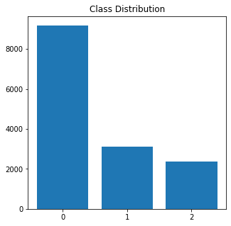
Understanding the class distribution
keys=['0','1','2']

# set figure size
plt.figure(figsize=(5,5))

# plot bat chart
plt.bar(keys,class_counts)

# set title
plt.title('Class Distribution')
import numpy as np
from sklearn.utils.class_weight import compute_class_weight
#class_weights = compute_class_weight('balanced', np.unique(labels), y=labels)
class_weights = compute_class_weight(class_weight = "balanced", classes= np.unique(labels), y= labels)
print("Class Weights:",class_weights)
Output
Class Weights: [0.54440912 1.471568 2.06782946]
# converting a list of class weights to a tensor
weights= torch.tensor(class_weights,dtype=torch.float)
# transfer to GPU
weights = weights.to(device)
# define the loss function
cross_entropy  = nn.NLLLoss(weight=weights)
#compute the loss
loss = cross_entropy(outputs, target)
print("Loss:",loss)
Output
import time
import datetime
# compute time in hh:mm:ss
def format_time(elapsed):
    # round to the nearest second.
    elapsed_rounded = int(round((elapsed)))
    # format as hh:mm:ss
    return str(datetime.timedelta(seconds = elapsed_rounded))
4.4 Model Training and Evaluation
Training: Epoch -> Batch -> Forward Pass -> Compute loss -> Backpropagate loss -> Update weights
Hence, for each epoch, we have training and validation phases. After each batch, we need to:
Training phase
- Load data onto the GPU for acceleration
- Unpack our data inputs and labels
- Clear out the gradients calculated in the previous pass.
- Forward pass (feed input data through the network)
- Backward pass (backpropagation)
- Update parameters with optimizer.step()
- Track variables for monitoring progress
#define a function for training the model
def train():

  print("\nTraining.....")

  #set the model on training phase - Dropout layers are activated
  model.train()

  #record the current time
  t0 = time.time()

  #initialize loss and accuracy to 0
  total_loss, total_accuracy = 0, 0

  #Create a empty list to save the model predictions
  total_preds=[]

  #for every batch
  for step,batch in enumerate(train_dataloader):

    # Progress update after every 40 batches.
    if step % 40 == 0 and not step == 0:

      # Calculate elapsed time in minutes.
      elapsed = format_time(time.time() - t0)

      # Report progress.
      print('  Batch {:>5,}  of  {:>5,}.    Elapsed: {:}.'.format(step, len(train_dataloader), elapsed))

    #push the batch to gpu
    batch = tuple(t.to(device) for t in batch)

    #unpack the batch into separate variables
    # `batch` contains three pytorch tensors:
    #   [0]: input ids
    #   [1]: attention masks
    #   [2]: labels
    sent_id, mask, labels = batch

    # Always clear any previously calculated gradients before performing a
    # backward pass. PyTorch doesn't do this automatically.
    model.zero_grad()

    # Perform a forward pass. This returns the model predictions
    preds = model(sent_id, mask)

    #compute the loss between actual and predicted values
    loss =  cross_entropy(preds, labels)

    # Accumulate the training loss over all of the batches so that we can
    # calculate the average loss at the end. `loss` is a Tensor containing a
    # single value; the `.item()` function just returns the Python value
    # from the tensor.
    total_loss = total_loss + loss.item()

    # Perform a backward pass to calculate the gradients.
    loss.backward()

    # Update parameters and take a step using the computed gradient.
    # The optimizer dictates the "update rule"--how the parameters are
    # modified based on their gradients, the learning rate, etc.
    optimizer.step()

    #The model predictions are stored on GPU. So, push it to CPU
    preds=preds.detach().cpu().numpy()

    #Accumulate the model predictions of each batch
    total_preds.append(preds)

  #compute the training loss of a epoch
  avg_loss     = total_loss / len(train_dataloader)

  #The predictions are in the form of (no. of batches, size of batch, no. of classes).
  #So, reshaping the predictions in form of (number of samples, no. of classes)
  total_preds  = np.concatenate(total_preds, axis=0)

  #returns the loss and predictions
  return avg_loss, total_preds
Evaluation: Epoch -> Batch -> Forward Pass -> Compute loss
Evaluation phase
- Load data onto the GPU for acceleration
- Unpack our data inputs and labels
- Forward pass (feed input data through the network)
- Compute loss on our validation data
- Track variables for monitoring progress
#define a function for evaluating the model
def evaluate():

  print("\nEvaluating.....")

  #set the model on training phase - Dropout layers are deactivated
  model.eval()

  #record the current time
  t0 = time.time()

  #initialize the loss and accuracy to 0
  total_loss, total_accuracy = 0, 0

  #Create a empty list to save the model predictions
  total_preds = []

  #for each batch
  for step,batch in enumerate(validation_dataloader):

    # Progress update every 40 batches.
    if step % 40 == 0 and not step == 0:

      # Calculate elapsed time in minutes.
      elapsed = format_time(time.time() - t0)

      # Report progress.
      print('  Batch {:>5,}  of  {:>5,}.    Elapsed: {:}.'.format(step, len(validation_dataloader), elapsed))

    #push the batch to gpu
    batch = tuple(t.to(device) for t in batch)

    #unpack the batch into separate variables
    # `batch` contains three pytorch tensors:
    #   [0]: input ids
    #   [1]: attention masks
    #   [2]: labels
    sent_id, mask, labels = batch

    #deactivates autograd
    with torch.no_grad():

      # Perform a forward pass. This returns the model predictions
      preds = model(sent_id, mask)

      #compute the validation loss between actual and predicted values
      loss = cross_entropy(preds,labels)

      # Accumulate the validation loss over all of the batches so that we can
      # calculate the average loss at the end. `loss` is a Tensor containing a
      # single value; the `.item()` function just returns the Python value
      # from the tensor.
      total_loss = total_loss + loss.item()

      #The model predictions are stored on GPU. So, push it to CPU
      preds=preds.detach().cpu().numpy()

      #Accumulate the model predictions of each batch
      total_preds.append(preds)

  #compute the validation loss of a epoch
  avg_loss = total_loss / len(validation_dataloader)

  #The predictions are in the form of (no. of batches, size of batch, no. of classes).
  #So, reshaping the predictions in form of (number of samples, no. of classes)
  total_preds  = np.concatenate(total_preds, axis=0)

  return avg_loss, total_preds
4.5 Train the Model
#Assign the initial loss to infinite
best_valid_loss = float('inf')

#create a empty list to store training and validation loss of each epoch
train_losses=[]
valid_losses=[]

epochs = 5

#for each epoch
for epoch in range(epochs):

    print('\n....... epoch {:} / {:} .......'.format(epoch + 1, epochs))

    #train model
    train_loss, _ = train()

    #evaluate model
    valid_loss, _ = evaluate()

    #save the best model
    if valid_loss < best_valid_loss:
        best_valid_loss = valid_loss
        torch.save(model.state_dict(), 'saved_weights.pt')

    #accumulate training and validation loss
    train_losses.append(train_loss)
    valid_losses.append(valid_loss)

    print(f'\nTraining Loss: {train_loss:.3f}')
    print(f'Validation Loss: {valid_loss:.3f}')

print("")
print("Training complete!")
Output
....... epoch 1 / 5 .......

Training.....
  Batch    40  of    391.    Elapsed: 0:00:02.
  Batch    80  of    391.    Elapsed: 0:00:05.
  Batch   120  of    391.    Elapsed: 0:00:07.
  Batch   160  of    391.    Elapsed: 0:00:09.
  Batch   200  of    391.    Elapsed: 0:00:12.
  Batch   240  of    391.    Elapsed: 0:00:14.
  Batch   280  of    391.    Elapsed: 0:00:17.
  Batch   320  of    391.    Elapsed: 0:00:19.
  Batch   360  of    391.    Elapsed: 0:00:21.

Evaluating.....
  Batch    40  of     44.    Elapsed: 0:00:02.

Training Loss: 1.098
Validation Loss: 1.088

....... epoch 2 / 5 .......

Training.....
  Batch    40  of    391.    Elapsed: 0:00:02.
  Batch    80  of    391.    Elapsed: 0:00:04.
  Batch   120  of    391.    Elapsed: 0:00:07.
  Batch   160  of    391.    Elapsed: 0:00:09.
  Batch   200  of    391.    Elapsed: 0:00:11.
  Batch   240  of    391.    Elapsed: 0:00:13.
  Batch   280  of    391.    Elapsed: 0:00:16.
  Batch   320  of    391.    Elapsed: 0:00:18.
  Batch   360  of    391.    Elapsed: 0:00:20.

Evaluating.....
  Batch    40  of     44.    Elapsed: 0:00:02.

Training Loss: 1.074
Validation Loss: 1.040

....... epoch 3 / 5 .......

Training.....
  Batch    40  of    391.    Elapsed: 0:00:02.
  Batch    80  of    391.    Elapsed: 0:00:04.
  Batch   120  of    391.    Elapsed: 0:00:06.
  Batch   160  of    391.    Elapsed: 0:00:09.
  Batch   200  of    391.    Elapsed: 0:00:11.
  Batch   240  of    391.    Elapsed: 0:00:13.
  Batch   280  of    391.    Elapsed: 0:00:15.
  Batch   320  of    391.    Elapsed: 0:00:17.
  Batch   360  of    391.    Elapsed: 0:00:19.

Evaluating.....
  Batch    40  of     44.    Elapsed: 0:00:02.

Training Loss: 1.056
Validation Loss: 1.040

....... epoch 4 / 5 .......

Training.....
  Batch    40  of    391.    Elapsed: 0:00:02.
  Batch    80  of    391.    Elapsed: 0:00:04.
  Batch   120  of    391.    Elapsed: 0:00:07.
  Batch   160  of    391.    Elapsed: 0:00:09.
  Batch   200  of    391.    Elapsed: 0:00:11.
  Batch   240  of    391.    Elapsed: 0:00:13.
  Batch   280  of    391.    Elapsed: 0:00:16.
  Batch   320  of    391.    Elapsed: 0:00:18.
  Batch   360  of    391.    Elapsed: 0:00:20.

Evaluating.....
  Batch    40  of     44.    Elapsed: 0:00:02.

Training Loss: 1.045
Validation Loss: 1.026

....... epoch 5 / 5 .......

Training.....
  Batch    40  of    391.    Elapsed: 0:00:02.
  Batch    80  of    391.    Elapsed: 0:00:04.
  Batch   120  of    391.    Elapsed: 0:00:07.
  Batch   160  of    391.    Elapsed: 0:00:09.
  Batch   200  of    391.    Elapsed: 0:00:11.
  Batch   240  of    391.    Elapsed: 0:00:13.
  Batch   280  of    391.    Elapsed: 0:00:16.
  Batch   320  of    391.    Elapsed: 0:00:18.
  Batch   360  of    391.    Elapsed: 0:00:20.

Evaluating.....
  Batch    40  of     44.    Elapsed: 0:00:02.

Training Loss: 1.038
Validation Loss: 1.010

Training complete!
4.6 Model Evaluation
# load weights of best model
path='saved_weights.pt'
model.load_state_dict(torch.load(path))
# get the model predictions on the validation data
# returns 2 elements- Validation loss and Predictions
valid_loss, preds = evaluate()
print(valid_loss)
Output
Evaluating.....
  Batch    40  of     44.    Elapsed: 0:00:02.
1.0100846696983685
from sklearn.metrics import classification_report
# Converting the log(probabities) into a classes
# Choosing index of a maximum value as class
y_pred = np.argmax(preds,axis=1)
# actual labels
y_true = validation_labels
print(classification_report(y_true,y_pred))
Output
              precision    recall  f1-score   support

           0       0.75      0.70      0.72       850
           1       0.39      0.34      0.36       314
           2       0.36      0.50      0.42       224

    accuracy                           0.59      1388
   macro avg       0.50      0.52      0.50      1388
weighted avg       0.60      0.59      0.59      1388
Conclusion
BERT has been a significant milestone in the field of natural language processing (NLP), particularly with the advent of Google AI language. Its impact spans across a spectrum of applications, from training language models to named entity recognition. Leveraging the encoder representations from transformers, BERT has revolutionized pre-trained models, enhancing their capabilities in understanding and processing textual data.
Machine learning techniques, particularly those involving natural language inference, have seen a notable advancement with the integration of BERT and similar models. These pre-trained BERT models have become instrumental in handling vast amounts of training data, pushing the boundaries of what’s achievable in NLP. The state-of-the-art techniques in language inference now heavily rely on the encoder mechanism, a core component of BERT
We have come to the end of the article. In brief, this article walked you through the transformer, BERT, and implementation of one of its use cases. Hope you enjoyed reading the blog. Feel free to use the comments section below or contact me on BERT to drop a query or feedback.


thanks for valuable info gcp training in hyderabad