State Space Search Optimization Using Local Search Algorithms
Introduction
Until now, we have seen two different approaches to state space search. i.e., Uninformed Search and Informed Search Strategies. These search strategies compute the path to the goal state from the initial state. A* Search Strategy is one of the best strategies which provides near-optimum solutions. It uses a heuristic and actual cost function to reach the goal state with minimum cost. To reach a goal state, It is important to have the cost function as minimum as possible.
In some problems, The path to the goal state is irrelevant. The only focus is to have a solution to reach the goal state. Hence, We are open to exploring all the possible solutions and reaching the goal state. The local search approach is one of the best ways to explore and evolve to reach the goal state. The local search algorithms examine and analyses many solutions (search space) by making local changes until an optimal solution is obtained or a no. of iterations are performed. Local Search Strategies are widely used for big problems and return a good solution.
Local search algorithms work by keeping a single “current” state or small set of states and iteratively trying to improve them. The best advantage of Local search is that we can control how much memory we use; hence, this is a very memory-efficient strategy. These strategies are highly used for examples like N-Queens, VLSI layout, and airline flight schedules.
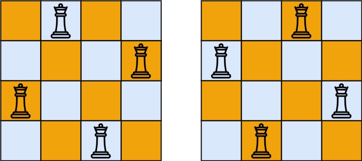
The n-queen problem is a viral chess-game challenge wherein the goal is to put n queens on an nxn board with no two queens attacking each other. (i.e., no two queens on the same diagonal or row or column)
This article was published as a part of the Data Science Blogathon.
(source: LeetCode)
What are Local Search Algorithms?
Local search algorithms are a class of optimization algorithms used to find solutions to optimization problems, particularly in situations where finding the globally optimal solution is impractical due to the size or complexity of the problem space. Instead of exploring the entire search space, local search algorithms focus on iteratively improving a candidate solution by making small, incremental changes.
At each step, the algorithm evaluates neighboring solutions to the current solution and selects the one that improves the objective function or meets certain criteria. These algorithms continue this process until a satisfactory solution is found or a termination condition is met.
Examples of local search algorithms include hill climbing, simulated annealing, and genetic algorithms. They are commonly used in various fields such as operations research, artificial intelligence, and computer science for solving problems like scheduling, routing, and resource allocation.
The Two famous Local Search Algorithms which we will be seeing in this article are:
1. Hill Climbing Algorithm
2. Genetic Algorithm
Hill Climbing Algorithm
The analogy:
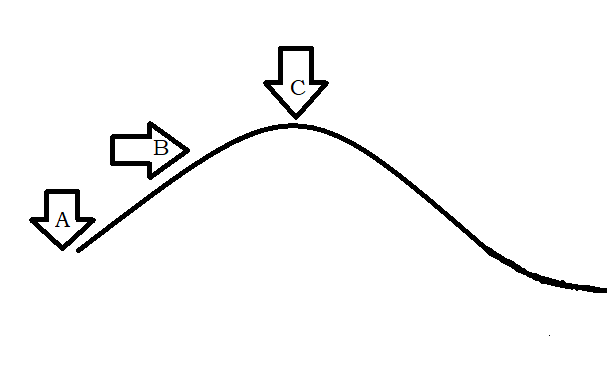
Consider that you want to climb a hill. However, there is a catch. Only once may you look at the top before the cloth is used to cover your eyes. What do you do then? You start walking in the direction of the top of the hill. You won’t change the direction in the middle as you may get lost on the hills. You will continue to ascend until you believe there is no more elevation to gain. That is, you are at the top of the hill. You stop when you sense a flat section or a downgrade. For instance, in the figure above, if someone were to start at position A and continue via position B to position C, they would eventually reach the top of the hill and stop there. The Hill Climbing algorithm, a local search algorithms, works analogously to this example.
About the Algorithm:
The algorithm works with the greedy approach. i.e., It moves in the direction which optimizes the cost. It follows the generate and test variant method without backtracking, as it does not record the previous states. Also, we do not need to maintain a tree or a graph for the states. Hill Climbing algorithms provide the best solution to the traveling salesman problem, where we need to minimize the distance traveled by the salesman.
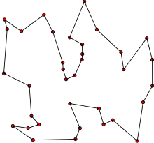
(source: Wikipedia/TSP)
The PseudoCode
function hill_climbing(problem)
{
        current = make_node(problem.initial_state)           //taking the initial node in current
        do{                                                //using a do while loop until returned
                  neighbor = highest valued successor of current   //considering only the highest valued successor of current
                  if value[neighbor] <= value[current]            //If its value is not better than the current node,
                            return current                       //we return the current node.                  current = neighbor                             //else, we make neighbor as current and loop again.
        }
}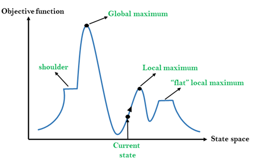
(source: javatpoint)
Understanding the hill climbing graph:
1. Local Maximum: One of the best solutions for the state space search, but a better solution exists.
2. Global Maximum: The best solution to the state space search problem.
3. shoulder: A plateau region where the algorithm stops assuming no better solution exists. But in reality, an uphill exists.
4. flat local maximum: Here, the neighbors have the same value; hence the algorithm stops.
Problems with the hill climbing algorithm:
1. Local Maxima: The algorithm stops at a local maximum, assuming it to be the best solution while a better solution exists.
2. Flat regions: The algorithm stops in the flat plateau regions as it assumes that this is the road ahead and an uphill doesn’t really exist.
3. Ridge: Here, every neighbor appears to be downhill, but the state space search has an uphill. The algorithm cannot change the direction and go uphill.
Genetic Algorithm
A Genetic algorithm is a local search technique used in computing to find true or approximate solutions to optimization and state space search problems. This algorithm is a class of evolutionary algorithms that uses techniques like inheritance, mutation, selection, and crossover inspired by evolutionary biology. The idea is taken from natural selection. i.e. Favourable traits become common and unfavorable traits become uncommon in successive generations. The solution is given by the survival of the fittest(Best solution).

Source: Quantdare
Understanding the terms of GA:
Individual: Any possible solution.
Population: Group of all individuals
Fitness: Each individual has a fitness value that helps determine the best solution.
Traits: Features of the individual.
How does this local search algorithms work?
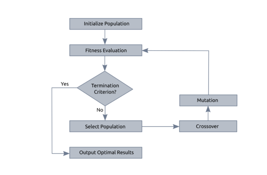
Step 1: Encode all the solutions to a problem in terms of the chromosome-like dataset.
Step 2: Evaluate the fitness function.
Step 3: Select Individuals(parents) for the next generation. (A parent with a good fitness score will help in evolving the offspring with a better fitness score.)
Step 4: Perform Mutation and crossover on different parents to produce new offspring.
Step 5: Evaluate their fitness function and repeat the process until the best solution is found.
What are Crossovers and Mutations?
Crossovers can be performed by selecting a binary substring of an individual and swapping it with a binary substring of the other individual. A mutation is performed by altering each gene with a probability.
The Flowchart:
(source: Artificial Intelligence: A Modern Approach book)
Local search optimization techniques, such as the Genetic Algorithm, are widely employed for tackling complex problems like the Traveling Salesman Problem and the Knapsack Problem. The Knapsack Problem revolves around optimizing the contents of a bag to maximize its value, given a defined weight constraint. Specifically, the challenge entails selecting items to pack into the bag so that the total value of the bag is maximized within the weight limit.

(source: AskPython)
“Genetic Algorithms are good at taking large, potentially huge search spaces and navigating them, looking for optimal combinations of things, solutions you might not otherwise find in a lifetime.”
– Salvatore Mangano
Conclusion
In this article, we learned about local search algorithms and understood 2 important algorithms. i.e. Hill climbing algorithm and Genetic algorithm. The key takeaways from this article are:
- While remaining true to its name, the Hill climbing algorithm is a blindfolded technique wherein the comparisons are made only with the neighbors to find the optimal solution.
- Hill climbing algorithms can sometimes land in problems when in the flat region or at the ridge, or the local maxima.
- Local search optimization, such as the genetic algorithm inspired by evolutionary biology, is one of the best approaches to ensure a solution.
- It follows Darvin’s natural selection theory, and only the fittest(best) survives(solution).
The media shown in this article is not owned by Analytics Vidhya and is used at the Author’s discretion.
