If you have been using GBM as a ‘black box’ till now, maybe it’s time for you to open it and see, how it actually works!
This article is inspired by Owen Zhang’s (Chief Product Officer at DataRobot and Kaggle Rank 3) approach shared at NYC Data Science Academy. He delivered a~2 hours talk and I intend to condense it and present the most precious nuggets here.
Boosting algorithms play a crucial role in dealing with bias variance trade-off. Unlike bagging algorithms, which only controls for high variance in a model, boosting controls both the aspects (bias & variance), and is considered to be more effective. A sincere understanding of GBM here should give you much needed confidence to deal with such critical issues.
In this article, I’ll disclose the science behind using GBM using Python. And, most important, how you can tune its parameters and obtain incredible results.
If you are completely new to the world of Ensemble learning, you can enrol in this free course which covers all the techniques in a structured manner: Ensemble Learning and Ensemble Learning Techniques
Special Thanks: Personally, I would like to acknowledge the timeless support provided by Mr. Sudalai Rajkumar, currently AV Rank 2. This article wouldn’t be possible without his guidance. I am sure the whole community will benefit from the same.
Complete Guide to Parameter Tuning in Gradient Boosting (GBM) in Python
Boosting is a sequential technique which works on the principle of ensemble. It combines a set of weak learners and delivers improved prediction accuracy. At any instant t, the model outcomes are weighed based on the outcomes of previous instant t-1. The outcomes predicted correctly are given a lower weight and the ones miss-classified are weighted higher. This technique is followed for a classification problem while a similar technique is used for regression.
Let’s understand it visually:
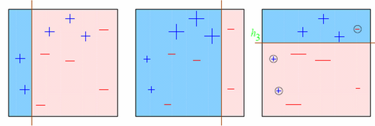
Observations:
Similar trend can be seen in box 3 as well. This continues for many iterations. In the end, all models are given a weight depending on their accuracy and a consolidated result is generated.
Did I whet your appetite? Good. Refer to these articles (focus on GBM right now):
The overall parameters of this ensemble model can be divided into 3 categories:
I’ll start with tree-specific parameters. First, lets look at the general structure of a decision tree:
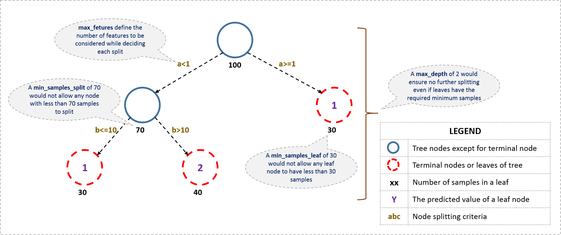
The parameters used for defining a tree are further explained below. Note that I’m using scikit-learn (python) specific terminologies here which might be different in other software packages like R. But the idea remains the same.
Before moving on to other parameters, lets see the overall pseudo-code of the GBM algorithm for 2 classes:
1. Initialize the outcome
2. Iterate from 1 to total number of trees
  2.1 Update the weights for targets based on previous run (higher for the ones mis-classified)
  2.2 Fit the model on selected subsample of data
  2.3 Make predictions on the full set of observations
  2.4 Update the output with current results taking into account the learning rate
3. Return the final output.
This is an extremely simplified (probably naive) explanation of GBM’s working. The parameters which we have considered so far will affect step 2.2, i.e. model building. Lets consider another set of parameters for managing boosting:
Apart from these, there are certain miscellaneous parameters which affect overall functionality:
I know its a long list of parameters but I have simplified it for you in an excel file which you can download from my GitHub repository.
We will take the dataset from Data Hackathon 3.x AV hackathon. The details of the problem can be found on the competition page. You can download the data set from here. I have performed the following steps:
For those who have the original data from competition, you can check out these steps from the data_preparation iPython notebook in the repository.
Lets start by importing the required libraries and loading the data:
Python Code:
Before proceeding further, lets define a function which will help us create GBM models and perform cross-validation.
def modelfit(alg, dtrain, predictors, performCV=True, printFeatureImportance=True, cv_folds=5):
    #Fit the algorithm on the data
    alg.fit(dtrain[predictors], dtrain['Disbursed'])

    #Predict training set:
    dtrain_predictions = alg.predict(dtrain[predictors])
    dtrain_predprob = alg.predict_proba(dtrain[predictors])[:,1]

    #Perform cross-validation:
    if performCV:
        cv_score = cross_validation.cross_val_score(alg, dtrain[predictors], dtrain['Disbursed'], cv=cv_folds, scoring='roc_auc')

    #Print model report:
    print "\nModel Report"
    print "Accuracy : %.4g" % metrics.accuracy_score(dtrain['Disbursed'].values, dtrain_predictions)
    print "AUC Score (Train): %f" % metrics.roc_auc_score(dtrain['Disbursed'], dtrain_predprob)

    if performCV:
        print "CV Score : Mean - %.7g | Std - %.7g | Min - %.7g | Max - %.7g" % (np.mean(cv_score),np.std(cv_score),np.min(cv_score),np.max(cv_score))

    #Print Feature Importance:
    if printFeatureImportance:
        feat_imp = pd.Series(alg.feature_importances_, predictors).sort_values(ascending=False)
        feat_imp.plot(kind='bar', title='Feature Importances')
        plt.ylabel('Feature Importance Score')
The code is pretty self-explanatory. Please feel free to drop a note in the comments if you find any challenges in understanding any part of it.
Lets start by creating a baseline model. In this case, the evaluation metric is AUC so using any constant value will give 0.5 as result. Typically, a good baseline can be a GBM model with default parameters, i.e. without any tuning. Lets find out what it gives:
#Choose all predictors except target & IDcols
predictors = [x for x in train.columns if x not in [target, IDcol]]
gbm0 = GradientBoostingClassifier(random_state=10)
modelfit(gbm0, train, predictors)

So, the mean CV score is 0.8319 and we should expect our model to do better than this.
As discussed earlier, there are two types of parameter to be tuned here – tree based and boosting parameters. There are no optimum values for learning rate as low values always work better, given that we train on sufficient number of trees.
Though, GBM is robust enough to not overfit with increasing trees, but a high number for a particular learning rate can lead to overfitting. But as we reduce the learning rate and increase trees, the computation becomes expensive and would take a long time to run on standard personal computers.
Keeping all this in mind, we can take the following approach:
In order to decide on boosting parameters, we need to set some initial values of other parameters. Lets take the following values:
Please note that all the above are just initial estimates and will be tuned later. Lets take the default learning rate of 0.1 here and check the optimum number of trees for that. For this purpose, we can do a grid search and test out values from 20 to 80 in steps of 10.
#Choose all predictors except target & IDcols
predictors = [x for x in train.columns if x not in [target, IDcol]]
param_test1 = {'n_estimators':range(20,81,10)}
gsearch1 = GridSearchCV(estimator = GradientBoostingClassifier(learning_rate=0.1, min_samples_split=500,min_samples_leaf=50,max_depth=8,max_features='sqrt',subsample=0.8,random_state=10),
param_grid = param_test1, scoring='roc_auc',n_jobs=4,iid=False, cv=5)
gsearch1.fit(train[predictors],train[target])
The output can be checked using following command:
gsearch1.grid_scores_, gsearch1.best_params_, gsearch1.best_score_
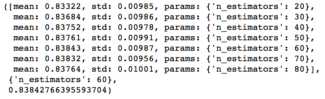
As you can see that here we got 60 as the optimal estimators for 0.1 learning rate. Note that 60 is a reasonable value and can be used as it is. But it might not be the same in all cases. Other situations:
Now lets move onto tuning the tree parameters. I plan to do this in following stages:
The order of tuning variables should be decided carefully. You should take the variables with a higher impact on outcome first. For instance, max_depth and min_samples_split have a significant impact and we’re tuning those first.
Important Note: I’ll be doing some heavy-duty grid searched in this section which can take 15-30 mins or even more time to run depending on your system. You can vary the number of values you are testing based on what your system can handle.
To start with, I’ll test max_depth values of 5 to 15 in steps of 2 and min_samples_split from 200 to 1000 in steps of 200. These are just based on my intuition. You can set wider ranges as well and then perform multiple iterations for smaller ranges.
param_test2 = {'max_depth':range(5,16,2), 'min_samples_split':range(200,1001,200)}
gsearch2 = GridSearchCV(estimator = GradientBoostingClassifier(learning_rate=0.1, n_estimators=60, max_features='sqrt', subsample=0.8, random_state=10),
param_grid = param_test2, scoring='roc_auc',n_jobs=4,iid=False, cv=5)
gsearch2.fit(train[predictors],train[target])
gsearch2.grid_scores_, gsearch2.best_params_, gsearch2.best_score_
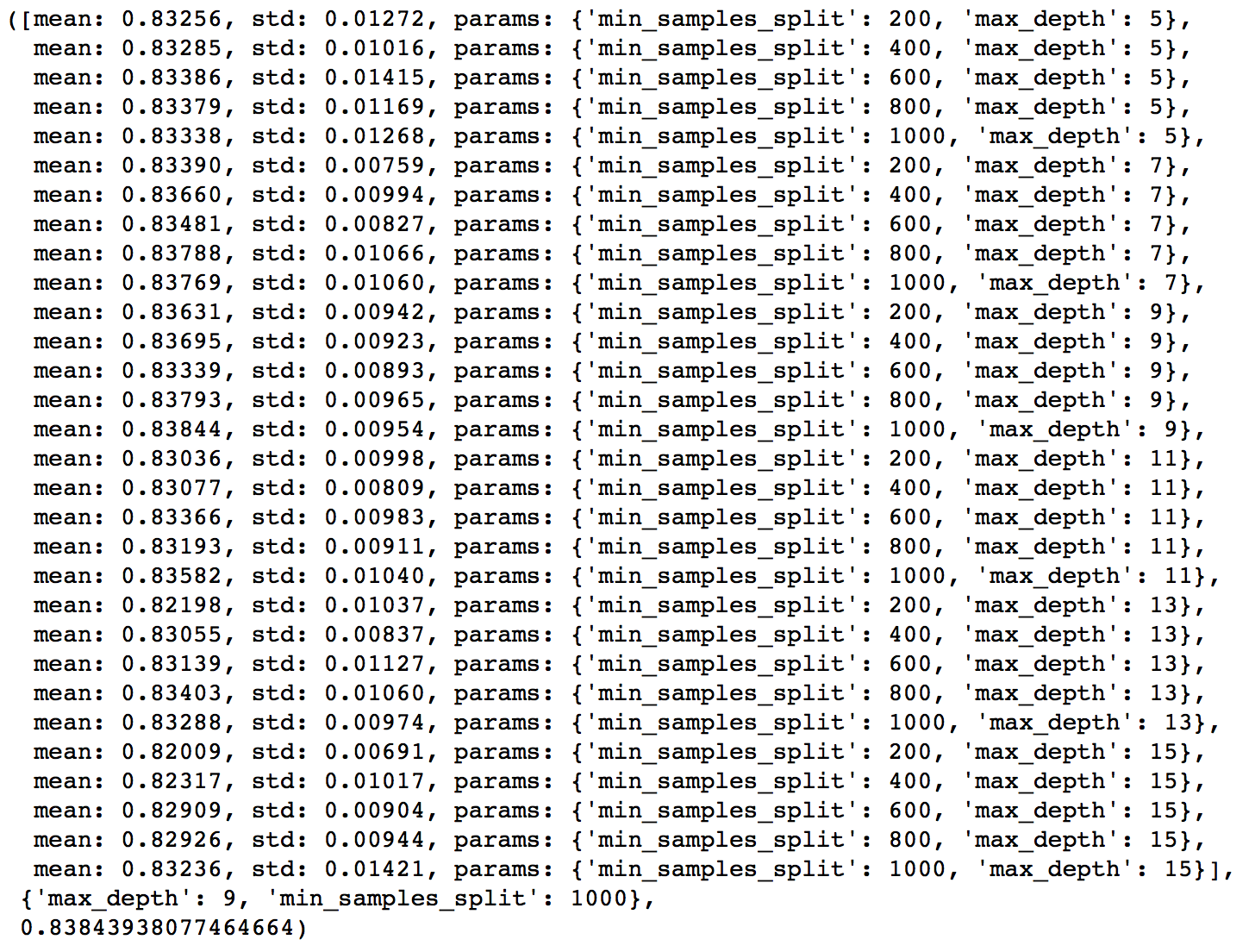
Here, we have run 30 combinations and the ideal values are 9 for max_depth and 1000 for min_samples_split. Note that, 1000 is an extreme value which we tested. There is a fare chance that the optimum value lies above that. So we should check for some higher values as well.
Here, I’ll take the max_depth of 9 as optimum and not try different values for higher min_samples_split. It might not be the best idea always but here if you observe the output closely, max_depth of 9 works better in most of the cases. Also, we can test for 5 values of min_samples_leaf, from 30 to 70 in steps of 10, along with higher min_samples_split.
param_test3 = {'min_samples_split':range(1000,2100,200), 'min_samples_leaf':range(30,71,10)}
gsearch3 = GridSearchCV(estimator = GradientBoostingClassifier(learning_rate=0.1, n_estimators=60,max_depth=9,max_features='sqrt', subsample=0.8, random_state=10),
param_grid = param_test3, scoring='roc_auc',n_jobs=4,iid=False, cv=5)
gsearch3.fit(train[predictors],train[target])
gsearch3.grid_scores_, gsearch3.best_params_, gsearch3.best_score_
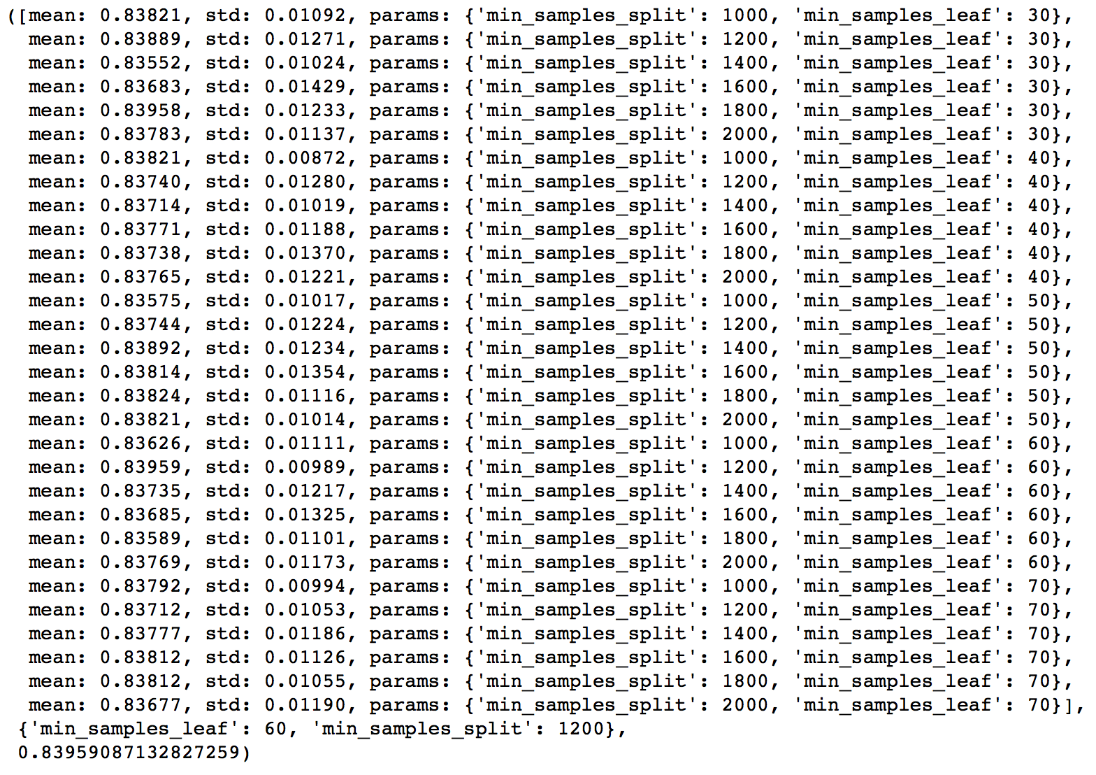
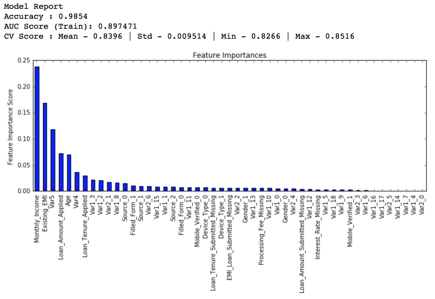
Here we get the optimum values as 1200 for min_samples_split and 60 for min_samples_leaf. Also, we can see the CV score increasing to 0.8396 now. Let’s fit the model again on this and have a look at the feature importance.
modelfit(gsearch3.best_estimator_, train, predictors)
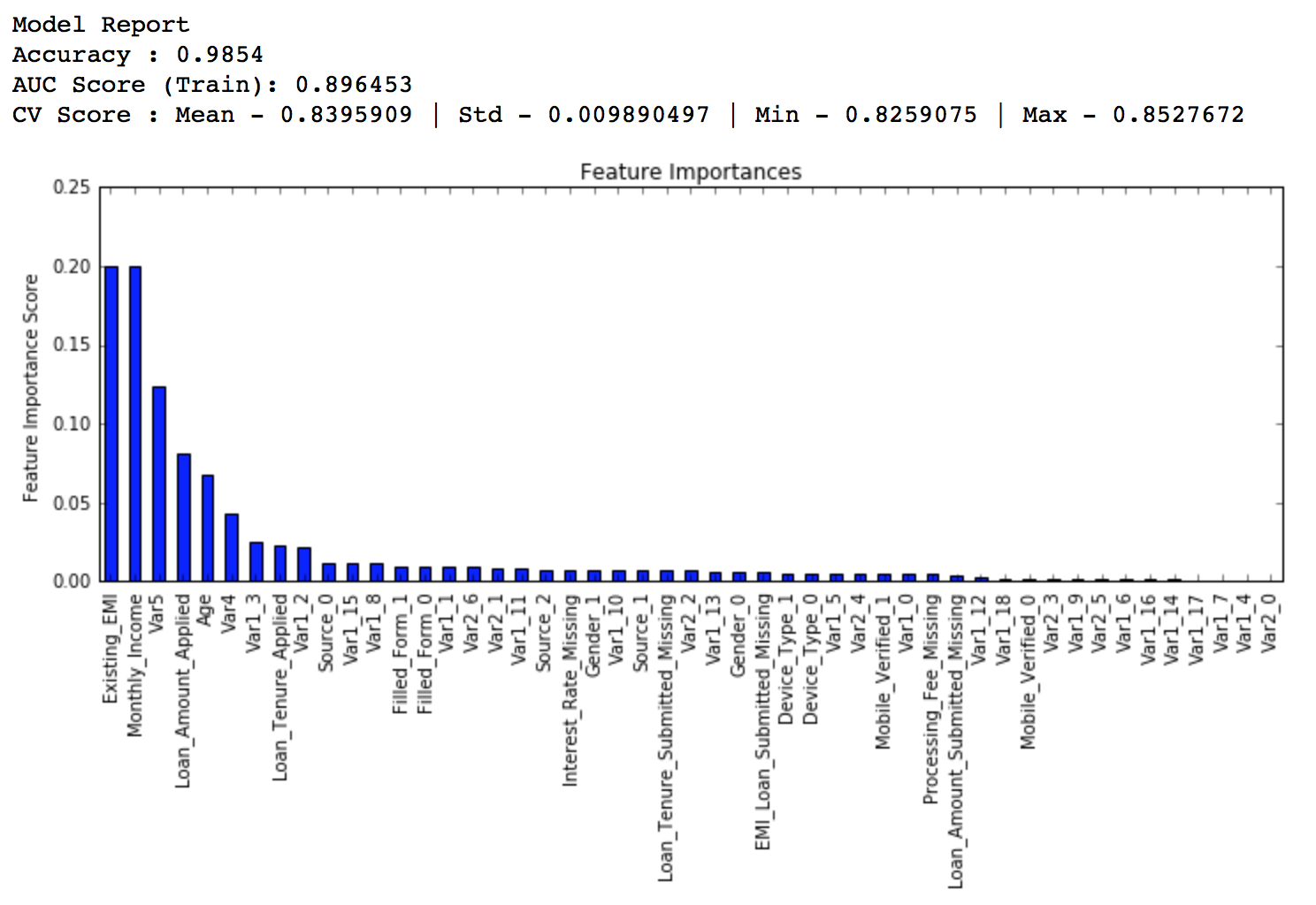
If you compare the feature importance of this model with the baseline model, you’ll find that now we are able to derive value from many more variables. Also, earlier it placed too much importance on some variables but now it has been fairly distributed.
Now lets tune the last tree-parameters, i.e. max_features by trying 7 values from 7 to 19 in steps of 2.
param_test4 = {'max_features':range(7,20,2)}
gsearch4 = GridSearchCV(estimator = GradientBoostingClassifier(learning_rate=0.1, n_estimators=60,max_depth=9, min_samples_split=1200, min_samples_leaf=60, subsample=0.8, random_state=10),
param_grid = param_test4, scoring='roc_auc',n_jobs=4,iid=False, cv=5)
gsearch4.fit(train[predictors],train[target])
gsearch4.grid_scores_, gsearch4.best_params_, gsearch4.best_score_
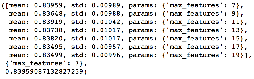
Here, we find that optimum value is 7, which is also the square root. So our initial value was the best. You might be anxious to check for lower values and you should if you like. I’ll stay with 7 for now. With this we have the final tree-parameters as:
The next step would be try different subsample values. Lets take values 0.6,0.7,0.75,0.8,0.85,0.9.
param_test5 = {'subsample':[0.6,0.7,0.75,0.8,0.85,0.9]}
gsearch5 = GridSearchCV(estimator = GradientBoostingClassifier(learning_rate=0.1, n_estimators=60,max_depth=9,min_samples_split=1200, min_samples_leaf=60, subsample=0.8, random_state=10,max_features=7),
param_grid = param_test5, scoring='roc_auc',n_jobs=4,iid=False, cv=5)
gsearch5.fit(train[predictors],train[target])
gsearch5.grid_scores_, gsearch5.best_params_, gsearch5.best_score_
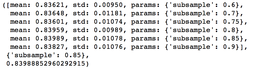
Here, we found 0.85 as the optimum value. Finally, we have all the parameters needed. Now, we need to lower the learning rate and increase the number of estimators proportionally. Note that these trees might not be the most optimum values but a good benchmark.
As trees increase, it will become increasingly computationally expensive to perform CV and find the optimum values. For you to get some idea of the model performance, I have included the private leaderboard scores for each. Since the data is not open, you won’t be able to replicate that but it’ll good for understanding.
Lets decrease the learning rate to half, i.e. 0.05 with twice (120) the number of trees.
predictors = [x for x in train.columns if x not in [target, IDcol]]
gbm_tuned_1 = GradientBoostingClassifier(learning_rate=0.05, n_estimators=120,max_depth=9, min_samples_split=1200,min_samples_leaf=60, subsample=0.85, random_state=10, max_features=7)
modelfit(gbm_tuned_1, train, predictors)
Private LB Score: 0.844139
Now lets reduce to one-tenth of the original value, i.e. 0.01 for 600 trees.
predictors = [x for x in train.columns if x not in [target, IDcol]]
gbm_tuned_2 = GradientBoostingClassifier(learning_rate=0.01, n_estimators=600,max_depth=9, min_samples_split=1200,min_samples_leaf=60, subsample=0.85, random_state=10, max_features=7)
modelfit(gbm_tuned_2, train, predictors)

Private LB Score: 0.848145
Lets decrease to one-twentieth of the original value, i.e. 0.005 for 1200 trees.
predictors = [x for x in train.columns if x not in [target, IDcol]]
gbm_tuned_3 = GradientBoostingClassifier(learning_rate=0.005, n_estimators=1200,max_depth=9, min_samples_split=1200, min_samples_leaf=60, subsample=0.85, random_state=10, max_features=7,
warm_start=True)
modelfit(gbm_tuned_3, train, predictors, performCV=False)
Private LB Score: 0.848112
Here we see that the score reduced very slightly. So lets run for 1500 trees.
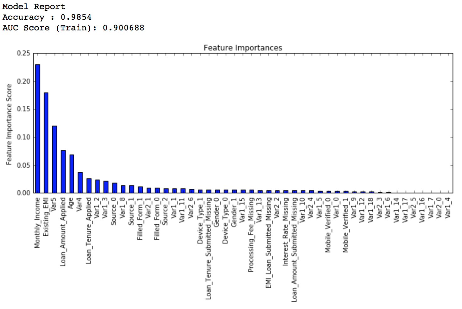
predictors = [x for x in train.columns if x not in [target, IDcol]]
gbm_tuned_4 = GradientBoostingClassifier(learning_rate=0.005, n_estimators=1500,max_depth=9, min_samples_split=1200, min_samples_leaf=60, subsample=0.85, random_state=10, max_features=7,
warm_start=True)
modelfit(gbm_tuned_4, train, predictors, performCV=False)

Private LB Score: 0.848747
Therefore, now you can clearly see that this is a very important step as private LB scored improved from ~0.844 to ~0.849 which is a significant jump.
Another hack that can be used here is the ‘warm_start’ parameter of GBM. You can use it to increase the number of estimators in small steps and test different values without having to run from starting always. You can also download the iPython notebook with all these model codes from my GitHub account.
This article was based on developing a GBM ensemble learning model end-to-end. We started with an introduction to boosting which was followed by detailed discussion on the various parameters involved. The parameters were divided into 3 categories namely the tree-specific, boosting and miscellaneous parameters depending on their impact on the model.
Finally, we discussed the general approach towards tackling a problem with GBM and also worked out the AV Data Hackathon 3.x problem through that approach.
I hope you found this useful and now you feel more confident to apply GBM in solving a data science problem. You can try this out in out upcoming signature hackathon Date Your Data.
Did you like this article? Would you like to share some other hacks which you implement while making GBM models? Please feel free to drop a note in the comments below and I’ll be glad to discuss.
Lorem ipsum dolor sit amet, consectetur adipiscing elit,


Great Article!! Can you do this for SVM,XGBoost, deep learning and neural networks.
Absolutely!! I plan to do an entire series if people like the first ones. XGBoost is definitely coming up next week.. There are a few others along with SVM and Deep Learning in my mind. But I haven't thought about a specific order yet.. Feel free to push in more suggestions.. It'll be easier for me to decide :) Also, it'll be great if you can share this article with others in your network. The more people read these, higher will be the preference we can set on articles of this kind!!
Wow great article, pretty much detailed and easy to understand. Am a great fan of articles posted on this site. Keep up the good work !
Thanks Jignesh :)
absolutely fantastic article. Loved the step by step approach. Would love to read more of these on SVM, deep learning. Also, it would be fantastic to have R code.
glad you liked it.. stay tuned for more!!
Guys, The article for XGBoost is out - http://www.analyticsvidhya.com/blog/2016/03/complete-guide-parameter-tuning-xgboost-with-codes-python/ I've also updated the same towards the end of this article. Enjoy and share your feedback! Cheers, Aarshay
Great example! One question; Where do you define 'dtrain'? I see it as an argument for the function.
Hi Don, Thanks for reaching out. So dtrain is a function argument and copies the passed value into dtrain. To explain further, a function is defined using following: def modelfit(alg, dtrain, predictors, performCV=True, printFeatureImportance=True, cv_folds=5): This tells that modelfit is a function which takes arguments as alg, dtrain, predictors and so on.. I need not define these arguments explicitly. When I call a function using: modelfit(gbm_tuned_4, train, predictors, performCV=False) The passed values get mapped to arguments. In this case: alg = gbm_tuned_4 dtrain =train predictors = predictors, and so on.. One this to note is that for some arguments I have defined a default value, like "performCV=True, printFeatureImportance=True, cv_folds=5". So you need not pass these always in a function. If not passed, the default values are taken. Cheers, Aarshay
Hi Aarshay, The article is simply superb. I have the following doubts.. Please clarify : 1. what is the difference between pylab and pyplot module in matplotlib library? (I searched in google and found certain results that pylab should not be used any further) can you please give some additional details what is the difference and which is preferred. 2. modelfit(gbm0,train,predictors,printOOB=False) is written by you at a specific place. modelfit does not accept 'printOOB' parameter. Can you please explain what is the use of this parameter?
Thanks Praveen! Regarding your concerns. 1. I didn't thought about this earlier but a quick search tells me that pyplot is the recommended option as you rightly mentioned. You can get some more intuition from this comment which I found online: "The pyplot interface is generally preferred for non-interactive plotting (i.e., scripting). The pylab interface is convenient for interactive calculations and plotting, as it minimizes typing. Note that this is what you get if you use the ipython shell with the -pylab option, which imports everything from pylab and makes plotting fully interactive." 2. I was using this earlier but I removed it later. I've updated the code with this removed. It was being used earlier to plot the OOB (out-of-bag) improvement curve. GBM returns OOB improvement scores which can be plotted to check how well the model is fitting. But later I found that the estimates provided are biased and many people recommend it should not be used. So I removed that plot from my codes.
That was amazing content, thanks for your efforts. What's your Kaggle account, if you don't mind sharing?
Thanks Jay.. Here is my kaggle account - https://www.kaggle.com/aarshayjain Even I am pretty new at Kaggle. This was my first serious participation..
Great article. Thank you so much for sharing. May I ask you some questions? 1.. You tuned the parameters with an order, first n_estimate and leraning_rate, then keep these parameters as the constants when you tuned other tree related parameters. Does the order really matter? I think it matters. But how did you figure out this order and what kinds of theories did you based on? 2. In sklearn, there is a tool called GridSearchCV. If we don't consider the cost of computing, we put every parameter together as a dict{ }, can we get a final, optimized set of parameters? I doubt it. What is your opinion? 3. Is your tuning method suitable for other datasets and other problems? Your response is highly appreciated. Thank you so much for your great work.
Amazing article! There is one small issue - in section Tuning tree-specific parameters the first stage called "Tune max_depth and num_samples_split", I guess it should be "min_samples_split"
And one more thing: "Here, I’ll take the max_depth of 9 as optimum and not try different values for higher min_samples_split" should be "Here, I’ll take the max_depth of 9 as optimum and NOW try different values for higher min_samples_split"
Great article. Thanks for sharing. One question: How do you adjust steps for parameter tuning? For instance you set 10 as step size for n_estimators paramater and found out that 60 has the highest CV accuracy. What if 55 provides significantly(!) better prediction accuracy and we missed it. Which approach should we follow to adjust step size? For example, should we try every number for integer parameter if computationally possible (10-20 hours maybe)? Thanks.
Hi, Please can you rename your variables in terms of X and y? Let X = training data(matrix) and y = target(a vector). I assume dtrain[predictors] = X and dtrain['Disbursed'] = y. In this section: #Print Feature Importance: if printFeatureImportance: feat_imp = pd.Series(alg.feature_importances_, predictors).sort_values(ascending=False) What is predictors? I know these questions sound basic but I'd really appreciate some help
Hey Aarshay, You said "The evaluation metric is AUC so using any constant value will give 0.5 as result. Typically, a good baseline can be a GBM model with default parameters," That's exactly what I encountered. I always got roc_auc_score of 0.5 even if I changed the parameters like n_estimators. I failed to get a baseline like 0.8 with default parameters. Part of my code is as follow. grd = GradientBoostingClassifier(random_state=10) grd.fit(X_train, y_train) score = roc_auc_score(y_test, grd.predict_proba(X_test)[:,1]) print (score) Do you think there's any problem? How can I get a higher auc score? Thanks a lot! Btw, I used different dataset with you.
Great article! My question is regarding to the max_depth: "Should be chosen (5-8) based on the number of observations and predictors. This has 87K rows and 49 columns so lets take 8 here." I want to know how 8 is calculated given 87K rows and 49 columns?
"If the value is around 20, you might want to try lowering the learning rate to 0.05 and re-run grid search" Can you please explain why you said so? if n-estimators is less, why would we decrease the learning rate?
hi, Thanks for it. Can you do this for R? I mean parameter tunig for GBM using R libraries please
Great Article
Hi. Great explanation. Just wanted to know while computing roc auc score why do you use dtrain_predprob instead of dtrain_predictions? Why not use the actual predictions while computing the roc-auc score?
I think you need to convert the String columns to int or float type first. I get this error when using the default code provided here: --------------------------------------------------------------------------- ValueError Traceback (most recent call last) in () 2 predictors = [x for x in train.columns if x not in [target, IDcol]] 3 gbm0 = GradientBoostingClassifier(random_state=10) ----> 4 modelfit(gbm0, train, predictors) in modelfit(alg, dtrain, predictors, performCV, printFeatureImportance, cv_folds) 1 def modelfit(alg, dtrain, predictors, performCV=True, printFeatureImportance=True, cv_folds=5): 2 #fit the algorithm on the data ----> 3 alg.fit(dtrain[predictors], dtrain['Disbursed']) 4 #predict on the training set 5 dtrain_predictions = alg.predict(dtrain[predictors]) ~\AppData\Local\Continuum\Anaconda3\envs\tensorflow\lib\site-packages\sklearn\ensemble\gradient_boosting.py in fit(self, X, y, sample_weight, monitor) 977 978 # Check input --> 979 X, y = check_X_y(X, y, accept_sparse=['csr', 'csc', 'coo'], dtype=DTYPE) 980 n_samples, self.n_features_ = X.shape 981 if sample_weight is None: ~\AppData\Local\Continuum\Anaconda3\envs\tensorflow\lib\site-packages\sklearn\utils\validation.py in check_X_y(X, y, accept_sparse, dtype, order, copy, force_all_finite, ensure_2d, allow_nd, multi_output, ensure_min_samples, ensure_min_features, y_numeric, warn_on_dtype, estimator) 571 X = check_array(X, accept_sparse, dtype, order, copy, force_all_finite, 572 ensure_2d, allow_nd, ensure_min_samples, --> 573 ensure_min_features, warn_on_dtype, estimator) 574 if multi_output: 575 y = check_array(y, 'csr', force_all_finite=True, ensure_2d=False, ~\AppData\Local\Continuum\Anaconda3\envs\tensorflow\lib\site-packages\sklearn\utils\validation.py in check_array(array, accept_sparse, dtype, order, copy, force_all_finite, ensure_2d, allow_nd, ensure_min_samples, ensure_min_features, warn_on_dtype, estimator) 431 force_all_finite) 432 else: --> 433 array = np.array(array, dtype=dtype, order=order, copy=copy) 434 435 if ensure_2d: ValueError: could not convert string to float: 'S122'
Hi Raj, Yes you need to convert string column to float.
Thank you for this amazing article. I have two questions. first, can we tune these hyperparameters using GPU ? because this is very time-consuming. The second one is when I implement this method on the costarica_poverty dataset the accuracy does not reduce by increasing the n-estimators (like what happened for you on 70 and 80 estimators) which is not good. and also after setting max_depth, num_samples_split and and min_samples_leaf I get accuracy = 1 and AUC score = 1. I would be very thank full if you show me a way to handle this.
thanks a lot for the article. I have two questions. first, can we tune these hyperparameters using GPU ? because this is very time-consuming. The second one is when I implement this method on the costarica_poverty dataset the accuracy does not reduce by increasing the n-estimators (like what happened for you on 70 and 80 estimators) which is not good. and also after setting max_depth, num_samples_split and and min_samples_leaf I get accuracy = 1 and AUC score = 1. I would be very thank full if you show me a way to handle this.