Learn Gradient Boosting Algorithm for better predictions (with codes in R)

Introduction

The accuracy of a predictive model can be boosted in two ways: Either by embracing feature engineering or by applying boosting algorithms straight away. Having participated in lots of data science competition, I’ve noticed that people prefer to work with boosting algorithms as it takes less time and produces similar results.

There are multiple boosting algorithms like Gradient Boosting, XGBoost, AdaBoost, Gentle Boost etc. Every algorithm has its own underlying mathematics and a slight variation is observed while applying them. If you are new to this, Great! You shall be learning all these concepts in a week’s time from now.

In this article, I’ve explained the underlying concepts and complexities of Gradient Boosting Algorithm. In addition, I’ve also shared an example to learn its implementation in R.

Note: This guide is meant for beginners. Hence, if you’ve already mastered this concept, you may skip this article here.

Quick Explanation

While working with boosting algorithms, you’ll soon come across two frequently occurring buzzwords: Bagging and Boosting. So, how are they different? Here’s a one line explanation:

Bagging: It is an approach where you take random samples of data, build learning algorithms and take simple means to find bagging probabilities.

Boosting: Boosting is similar, however the selection of sample is made more intelligently. We subsequently give more and more weight to hard to classify observations.

Okay! I understand you’ve questions sprouting up like ‘what do you mean by hard? How do I know how much additional weight am I supposed to give to a mis-classified observation.’ I shall answer all your questions in subsequent sections. Keep Calm and proceed.

Let’s begin with an easy example

Assume, you are given a previous model M to improve on. Currently you observe that the model has an accuracy of 80% (any metric). How do you go further about it?

One simple way is to build an entirely different model using new set of input variables and trying better ensemble learners. On the contrary, I have a much simpler way to suggest. It goes like this:

Y = M(x) + error

What if I am able to see that error is not a white noise but have same correlation with outcome(Y) value. What if we can develop a model on this error term? Like,

error = G(x) + error2

Probably, you’ll see error rate will improve to a higher number, say 84%. Let’s take another step and regress against error2.

error2 = H(x) + error3

Now we combine all these together :

Y = M(x) + G(x) + H(x) + error3

This probably will have a accuracy of even more than 84%. What if I can find an optimal weights for each of the three learners,

Y = alpha * M(x) + beta * G(x) + gamma * H(x) + error4

If we found good weights, we probably have made even a better model. This is the underlying principle of a boosting learner. When I read the theory for the first time, I had two quick questions:

1. Do we really see non white noise error in regression/classification equations? If not, how can we even use this algorithm?
2. Wow, if this is possible, why not get near 100% accuracy?

I’ll answer these questions in this article, however, in a crisp manner. Boosting is generally done on weak learners, which do not have a capacity to leave behind white noise.  Secondly, boosting can lead to overfitting, so we need to stop at the right point.

Let’s try to visualize one Classification Problem

Look at the below diagram :

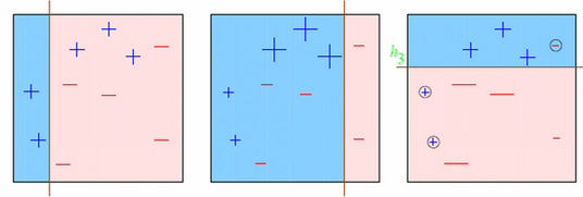
We start with the first box. We see one vertical line which becomes our first week learner. Now in total we have 3/10 mis-classified observations. We now start giving higher weights to 3 plus mis-classified observations. Now, it becomes very important to classify them right. Hence, the vertical line towards right edge. We repeat this process and then combine each of the learner in appropriate weights.

Explaining underlying mathematics

How do we assign weight to observations?

We always start with a uniform distribution assumption. Lets call it as D1 which is 1/n for all n observations.

Step 1 . We assume an alpha(t)

Step 2: Get a weak classifier h(t)

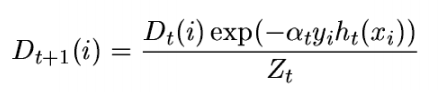
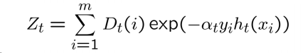
Step 3: Update the population distribution for the next step

where,

Step 4 : Use the new population distribution to again find the next learner

Scared of Step 3 mathematics? Let me break it down for you. Simply look at the argument in exponent. Alpha is kind of learning rate, y is the actual response ( + 1 or -1) and h(x) will be the class predicted by learner. Essentially, if learner is going wrong, the exponent becomes 1*alpha and else -1*alpha. Essentially, the weight will probably increase if the prediction went wrong the last time. So, what’s next?

Step 5 : Iterate step 1 – step 4 until no hypothesis is found which can improve further.

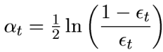
Step 6 : Take a weighted average of the frontier using all the learners used till now. But what are the weights? Weights are simply the alpha values. Alpha is calculated as follows:

Time to Practice – Example

I recently participated in an online hackathon organized by Analytics Vidhya. For making the variable transformation easier, I combined both test and train data in the file complete_data. I started with basic import function and splitted the population in Devlopment, ITV and Scoring.

library(caret)
rm(list=ls())
setwd("C:\\Users\\ts93856\\Desktop\\AV")
library(Metrics)

complete <- read.csv("complete_data.csv", stringsAsFactors = TRUE)
train <- complete[complete$Train == 1,]
score <- complete[complete$Train != 1,]

set.seed(999)

ind <- sample(2, nrow(train), replace=T, prob=c(0.60,0.40))
trainData<-train[ind==1,]
testData <- train[ind==2,]

set.seed(999)
ind1 <- sample(2, nrow(testData), replace=T, prob=c(0.50,0.50))
trainData_ens1<-testData[ind1==1,]
testData_ens1 <- testData[ind1==2,]

table(testData_ens1$Disbursed)[2]/nrow(testData_ens1)
#Response Rate of 9.052%

Here is all you need to do, to build a GBM model.

fitControl <- trainControl(method = "repeatedcv", number = 4, repeats = 4)

trainData$outcome1 <- ifelse(trainData$Disbursed == 1, "Yes","No")
set.seed(33)
gbmFit1 <- train(as.factor(outcome1) ~ ., data = trainData[,-26], method = "gbm", trControl = fitControl,verbose = FALSE)

gbm_dev <- predict(gbmFit1, trainData,type= "prob")[,2] 
gbm_ITV1 <- predict(gbmFit1, trainData_ens1,type= "prob")[,2] 
gbm_ITV2 <- predict(gbmFit1, testData_ens1,type= "prob")[,2]

auc(trainData$Disbursed,gbm_dev)
auc(trainData_ens1$Disbursed,gbm_ITV1)
auc(testData_ens1$Disbursed,gbm_ITV2)

As you will see after running this code, all AUC will come extremely close to 0.84 . I will leave the feature engineering upto you, as the competition is still on. You are welcome to use this code to compete though. GBM is the most widely used algorithm. XGBoost is another faster version of boosting learner which I will cover in any future articles.

End Notes

I have seen boosting learners extremely quick and highly efficient. They have never disappointed me to get high initial scores on Kaggle and other platforms. However, it all boils down to how well can you do feature engineering.

Have you used Gradient Boosting before? How did the model perform? Have you used boosting learners in any other capacity. If yes, I would love to hear your experiences in the comments section below.

If you like what you just read & want to continue your analytics learning, subscribe to our emails, follow us on twitter or like our facebook page

Tavish Srivastava

Tavish Srivastava, co-founder and Chief Strategy Officer of Analytics Vidhya, is an IIT Madras graduate and a passionate data-science professional with 8+ years of diverse experience in markets including the US, India and Singapore, domains including Digital Acquisitions, Customer Servicing and Customer Management, and industry including Retail Banking, Credit Cards and Insurance. He is fascinated by the idea of artificial intelligence inspired by human intelligence and enjoys every discussion, theory or even movie related to this idea.