Mastering XGBoost Parameters Tuning: A Complete Guide with Python Codes
If things don’t go your way in predictive modeling, use XGboost. XGBoost algorithm has become the ultimate weapon of many data scientists. It’s a highly sophisticated algorithm, powerful enough to deal with all sorts of irregularities of data. It uses parallel computation in which multiple decision trees are trained in parallel to find the final prediction. This article is best suited to people who are new to XGBoost. We’ll learn the art of XGBoost parameters tuning and XGBoost hyperparameter tuning. Also, we’ll practice this algorithm using a training data set in Python.
Table of contents
What is XGBoost?
Building a machine learning model using the XGBoost classifier is a straightforward process. Naturally, XGBoost simplifies the initial model creation. However, enhancing the model’s performance through XGBoost can be challenging—personally, I encountered some struggles in this phase. This algorithm involves various parameters, and achieving an optimized model requires meticulous parameter tuning. Determining the right set of parameters to fine-tune can be perplexing, and discerning the ideal values for these parameters is crucial for obtaining the best possible output. Consequently, obtaining practical answers to questions such as which parameters to focus on and what values to assign becomes a complex aspect of refining an XGBoost model.
XGBoost (eXtreme Gradient Boosting) is an advanced implementation of a gradient boosting algorithm, which has gained popularity for its high performance and efficiency in various machine learning tasks. If you are already familiar with Gradient Boosting Machine (GBM), you may find it insightful to delve into XGBoost’s naturally extensive set of parameters. I previously provided an in-depth exploration of parameter tuning for GBM in my article titled “Complete Guide to Parameter Tuning in Gradient Boosting (GBM) in Python.” I highly recommend reviewing that material before proceeding further, as it will not only enhance your overall understanding of boosting techniques but also prepare you for a more nuanced comprehension of naturally available XGBoost parameters.
Sample Project to Apply XGBoostProblem StatementHR analytics is revolutionizing the way human resources departments operate, leading to higher efficiency and better results overall. Human resources have been using analytics for years.However, the collection, processing, and analysis of data have been largely manual, and given the nature of human resources dynamics and HR KPIs, the approach has been constraining HR. Therefore, it is surprising that HR departments woke up to the utility of machine learning so late in the game. Here is an opportunity to try predictive analytics in identifying the employees most likely to get promoted. Practice Now
Advantages of XGBoost
I’ve always admired the boosting capabilities that the XGBoost parameters algorithm infuses into a predictive model. When I explored more about its performance and the science behind its high accuracy, I discovered many advantages, including the flexibility and power of its parameters :
Regularization
Standard GBM implementation has no regularization like XGBoost; therefore, it also helps to reduce overfitting. In fact, XGBoost is also known as a ‘regularized boosting‘ technique.
Parallel Processing
XGBoost implements parallel processing and is blazingly faster as compared to GBM.
But hang on, we know that boosting is a sequential process so how can it be parallelized? We know that each tree can be built only after the previous one, so what stops us from making a tree using all cores? I hope you get where I’m coming from. Check this link out to explore further. XGBoost also supports implementation on Hadoop.
High Flexibility
XGBoost allows users to define custom optimization objectives and evaluation criteria. This adds a whole new dimension to the model and there is no limit to what we can do.
Handling Missing Values
XGBoost has an in-built routine to handle missing values. The user is required to supply a different value than other observations and pass that as a parameter. XGBoost tries different things as it encounters a missing value on each node and learns which path to take for missing values in the future.
Tree Pruning
A GBM would stop splitting a node when it encounters a negative loss in the split. Thus it is more of a greedy algorithm. XGBoost parameters, on the other hand, makes splits up to the max_depth specified and then starts pruning the tree backward and removing splits beyond which there is no positive gain.
Another advantage is that sometimes a split of negative loss, say -2, may be followed by a split of positive loss +10. GBM would stop as it encounters -2. But XGBoost will go deeper, and it will see a combined effect of +8 of the split and keep both.
Built-in Cross-Validation
XGBoost allows the user to run a cross-validation at each iteration of the boosting process and thus, it is easy to get the exact optimum number of boosting iterations in a single run. This is unlike GBM, where we have to run a grid search, and only limited values can be tested.
Continue on the Existing Model
Users can start training an XGBoost parameters model from its last iteration of the previous run. This can be of significant advantage in certain specific applications. GBM implementation of sklearn also has this feature, so they are even on this point.
I hope now you understand the sheer power XGBoost algorithm. Note that these are the points that I could muster. Do you know a few more? Feel free to drop a comment below, and I will update the list.
What are XGBoost Parameters?
The overall parameters have been divided into 3 categories by XGBoost authors:
- General Parameters: Guide the overall functioning
- Booster Parameters: Guide the individual booster (tree/regression) at each step
- Learning Task Parameters: Guide the optimization performed
Must Read: Complete Machine Learning Guide to Parameter Tuning in Gradient Boosting (GBM) in Python
General Parameters
These define the overall functionality of XGBoost.
- booster [default=gbtree]
- Select the type of model to run at each iteration. It has 2 options:
- gbtree: tree-based models
- gblinear: linear models
- Select the type of model to run at each iteration. It has 2 options:
- silent [default=0]
- Silent mode is activated is set to 1, i.e., no running messages will be printed.
- It’s generally good to keep it 0 as the messages might help in understanding the model.
- nthread [default to the maximum number of threads available if not set]
- This is used for parallel processing, and the number of cores in the system should be entered
- If you wish to run on all cores, the value should not be entered, and the algorithm will detect it automatically
There are 2 more parameters that are set automatically by XGBoost, and you need not worry about them. Let’s move on to Booster parameters.
Booster Parameters
Though there are 2 types of boosters, I’ll consider only tree booster here because it always outperforms the linear booster, and thus the latter is rarely used.
| Parameter | Description | Typical Values |
|---|---|---|
| eta | Analogous to the learning rate in GBM. | 0.01-0.2 |
| min_child_weight | Defines the minimum sum of weights of observations required in a child. | Tuned using CV |
| max_depth | The maximum depth of a tree. Used to control over-fitting. | 3-10 |
| max_leaf_nodes | The maximum number of terminal nodes or leaves in a tree. | |
| gamma | Specifies the minimum loss reduction required to make a split. | Tuned depending on loss function |
| max_delta_step | Allows each tree’s weight estimation to be constrained. | Usually not needed, explore if necessary |
| subsample | Denotes the fraction of observations to be random samples for each tree. | 0.5-1 |
| colsample_bytree | Denotes the fraction of columns to be random samples for each tree. | 0.5-1 |
| colsample_bylevel | Denotes the subsample ratio of columns for each split in each level. | Usually not used |
| lambda | L2 regularization term on weights (analogous to Ridge regression). | Explore for reducing overfitting |
| alpha | L1 regularization term on weight (analogous to Lasso regression). | Used for high dimensionality |
| scale_pos_weight | Used in case of high-class imbalance for faster convergence. | > 0 |
Learning Task Parameters
These parameters are used to define the optimization objective and the metric to be calculated at each step.
- objective [default=reg:linear]
- This defines the loss function to be minimized. Mostly used values are:
- binary: logistic –logistic regression for binary classification returns predicted probability (not class)
- multi: softmax –multiclass classification using the softmax objective, returns predicted class (not probabilities)
- you also need to set an additional num_class (number of classes) parameter defining the number of unique classes
- multi: softprob –same as softmax, but returns predicted probability of each data point belonging to each class.
- This defines the loss function to be minimized. Mostly used values are:
- eval_metric [ default according to objective ]
- The evaluation metrics are to be used for validation data.
- The default values are rmse for regression and error for classification.
- Typical values are:
- rmse – root mean square error
- mae – mean absolute error
- logloss – negative log-likelihood
- error – Binary classification error rate (0.5 thresholds)
- merror – Multiclass classification error rate
- mlogloss – Multiclass logloss
- auc: Area under the curve
- seed [default=0]
- The random number seed.
- It can be used for generating reproducible results and also for parameter tuning.
If you’ve been using Scikit-Learn till now, these parameter names might not look familiar. The good news is that the xgboost module in python has an sklearn wrapper called XGBClassifier parameters. It uses the sklearn style naming convention. The parameters names that will change are:
- eta –> learning_rate
- lambda –> reg_lambda
- alpha –> reg_alpha
You must be wondering why we have defined everything except something similar to the “n_estimators” parameter in GBM. Well, this exists as a parameter in XGBClassifier. However, it has to be passed as “num_boosting_rounds” while calling the fit function in the standard xgboost implementation.
Go through the following parts of the xgboost guide to better understand the parameters and codes:
- XGBoost Parameters (official guide)
- XGBoost Demo Codes (xgboost GitHub repository)
- Python API Reference (official guide)
XGBoost Parameters Tuning With Example
We will take the data set from Data Hackathon 3.x AV hackathon, as taken in the GBM article. The details of the problem can be found on the competition page. You can download the data set from here. I have performed the following steps:
- The city variable dropped because of too many categories.
- DOB converted to Age | DOB dropped.
- EMI_Loan_Submitted_Missing created, which is 1 if EMI_Loan_Submitted was missing; else 0 | Original variable EMI_Loan_Submitted dropped.
- EmployerName dropped because of too many categories.
- Existing_EMI imputed with 0 (median) since only 111 values were missing.
- Interest_Rate_Missing created, which is 1 if Interest_Rate was missing; else 0 | Original variable Interest_Rate dropped.
- Lead_Creation_Date dropped because it made a little intuitive impact on the outcome.
- Loan_Amount_Applied, Loan_Tenure_Applied imputed with median values.
- Loan_Amount_Submitted_Missing created, which is 1 if Loan_Amount_Submitted was missing; else 0 | Original variable Loan_Amount_Submitted dropped.
- Loan_Tenure_Submitted_Missing created, which is 1 if Loan_Tenure_Submitted was missing; else 0 | Original variable Loan_Tenure_Submitted dropped.
- LoggedIn, Salary_Account dropped.
- Processing_Fee_Missing created, which is 1 if Processing_Fee was missing; else 0 | Original variable Processing_Fee dropped.
- Source – top 2 kept as is, and all others are combined into a different category.
- Numerical and One-Hot-Coding performed.
For those who have the original data from the competition, you can check out these steps from the data_preparation iPython notebook in the repository.
Let’s start by importing the required libraries and loading the data.
Python Code
Note that I have imported 2 forms of XGBoost:
- xgb – this is the direct xgboost library. I will use a specific function, “cv” from this library
- XGBClassifier – this is an sklearn wrapper for XGBoost. This allows us to use sklearn’s Grid Search with parallel processing in the same way we did for GBM.
Before proceeding further, let’s define a function that will help us create XGBoost models and perform cross-validation. The best part is that you can take this function as it is and use it later for your own models.
def modelfit(alg, dtrain, predictors,useTrainCV=True, cv_folds=5, early_stopping_rounds=50):

    if useTrainCV:
        xgb_param = alg.get_xgb_params()
        xgtrain = xgb.DMatrix(dtrain[predictors].values, label=dtrain[target].values)
        cvresult = xgb.cv(xgb_param, xgtrain, num_boost_round=alg.get_params()['n_estimators'], nfold=cv_folds,
            metrics='auc', early_stopping_rounds=early_stopping_rounds, show_progress=False)
        alg.set_params(n_estimators=cvresult.shape[0])

    #Fit the algorithm on the data
    alg.fit(dtrain[predictors], dtrain['Disbursed'],eval_metric='auc')

    #Predict training set:
    dtrain_predictions = alg.predict(dtrain[predictors])
    dtrain_predprob = alg.predict_proba(dtrain[predictors])[:,1]

    #Print model report:
    print "\nModel Report"
    print "Accuracy : %.4g" % metrics.accuracy_score(dtrain['Disbursed'].values, dtrain_predictions)
    print "AUC Score (Train): %f" % metrics.roc_auc_score(dtrain['Disbursed'], dtrain_predprob)

    feat_imp = pd.Series(alg.booster().get_fscore()).sort_values(ascending=False)
    feat_imp.plot(kind='bar', title='Feature Importances')
    plt.ylabel('Feature Importance Score')
This code is slightly different from what I used for GBM. The focus of this article is to cover the concepts and not coding. Please feel free to drop a note in the comments if you find any challenges in understanding any part of it. Note that xgboost’s sklearn wrapper doesn’t have a “feature_importances” metric but a get_fscore() function, which does the same job.
General Approach for XGBoost Parameters Tuning
We will use an approach similar to that of GBM here. The various steps to be performed are:
- Choose a relatively high learning rate. Generally, a learning rate of 0.1 works, but somewhere between 0.05 to 0.3 should work for different problems. Determine the optimum number of trees for this learning rate. XGBoost has a very useful function called “cv” which performs cross-validation at each boosting iteration and thus returns the optimum number of trees required.
- Tune tree-specific parameters ( max_depth, min_child_weight, gamma, subsample, colsample_bytree) for the decided learning rate and the number of trees. Note that we can choose different parameters to define a tree, and I’ll take up an example here.
- Tune regularization parameters (lambda, alpha) for xgboost, which can help reduce model complexity and enhance performance.
- Lower the learning rate and decide the optimal parameters.
Let us look at a more detailed step-by-step approach.
Step 1: Fix the learning rate and number of estimators for tuning tree-based parameters.
In order to decide on boosting parameters, we need to set some initial values of other parameters. Let’s take the following values:
- max_depth = 5: This should be between 3-10. I’ve started with 5, but you can choose a different number as well. 4-6 can be good starting points.
- min_child_weight = 1: A smaller value is chosen because it is a highly imbalanced class problem, and leaf nodes can have smaller size groups.
- gamma = 0: A smaller value like 0.1-0.2 can also be chosen for starting. This will, anyways, be tuned later.
- subsample, colsample_bytree = 0.8: This is a commonly used start value. Typical values range between 0.5-0.9.
- scale_pos_weight = 1: Because of high-class imbalance.
Please note that all the above are just initial estimates and will be tuned later. Let’s take the default learning rate of 0.1 here and check the optimum number of trees using the cv function of xgboost. The function defined above will do it for us.
#Choose all predictors except target & IDcols
predictors = [x for x in train.columns if x not in [target, IDcol]]
xgb1 = XGBClassifier(
 learning_rate =0.1,
 n_estimators=1000,
 max_depth=5,
 min_child_weight=1,
 gamma=0,
 subsample=0.8,
 colsample_bytree=0.8,
 objective= 'binary:logistic',
 nthread=4,
 scale_pos_weight=1,
 seed=27)
modelfit(xgb1, train, predictors)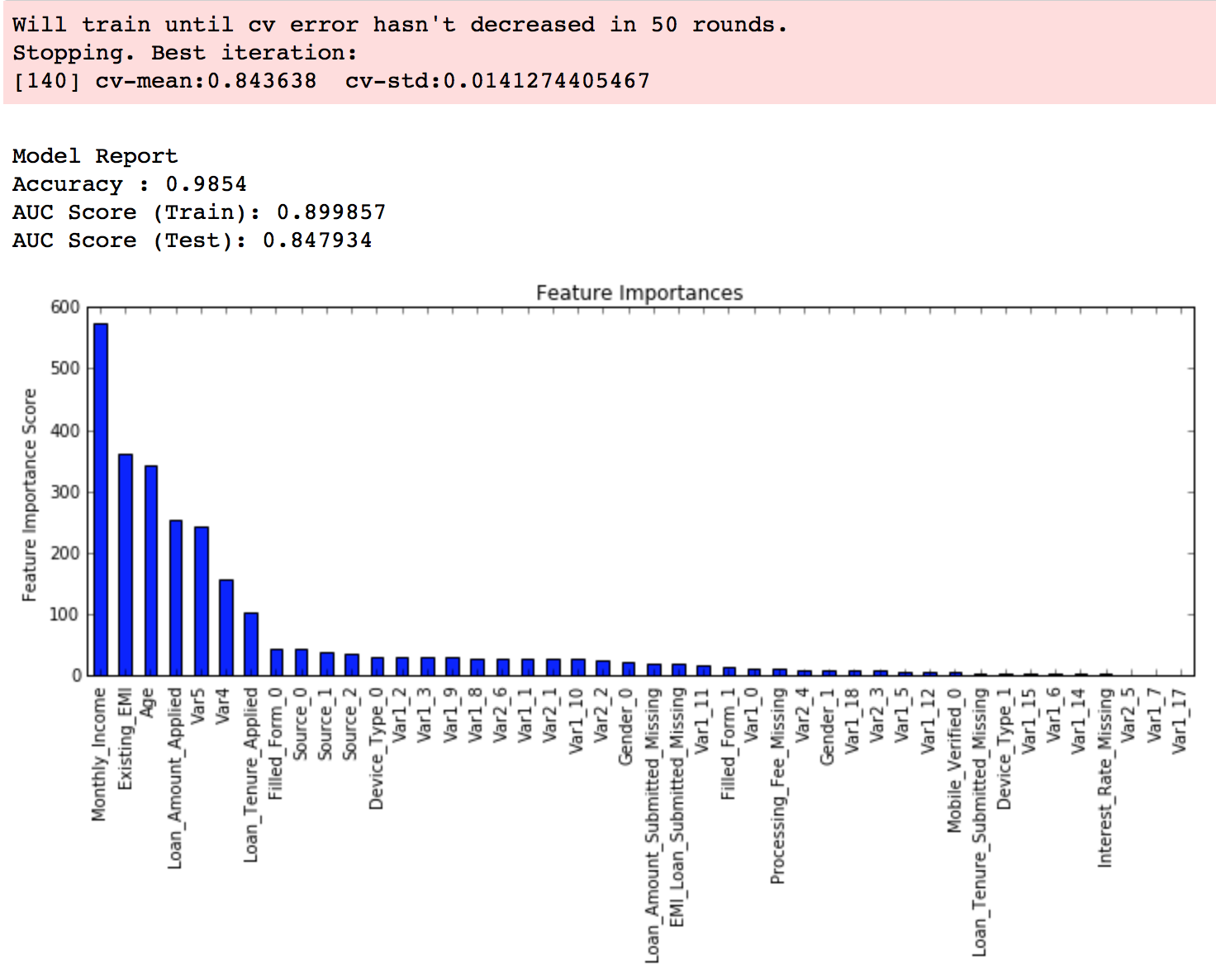
As you can see that here we got 140 as the optimal estimator for a 0.1 learning rate. Note that this value might be too high for you depending on your system’s power. In that case, you can increase the learning rate and re-run the command to get the reduced number of estimators.
Note: You will see the test AUC as “AUC Score (Test)” in the outputs here. But this would not appear if you try to run the command on your system as the data is not made public. It’s provided here just for reference. The part of the code which generates this output has been removed here.
Step 2: Tune max_depth and min_child_weight.
We tune these first as they will have the highest impact on the model outcome. To start with, let’s set wider ranges, and then we will perform another iteration for smaller ranges.
Important Note: I’ll be doing some heavy-duty grid searches in this section, which can take 15-30 mins or even more time to run, depending on your system. You can vary the number of values you are testing based on what your system can handle.
param_test1 = {
 'max_depth':range(3,10,2),
 'min_child_weight':range(1,6,2)
}
gsearch1 = GridSearchCV(estimator = XGBClassifier( learning_rate =0.1, n_estimators=140, max_depth=5,
 min_child_weight=1, gamma=0, subsample=0.8, colsample_bytree=0.8,
 objective= 'binary:logistic', nthread=4, scale_pos_weight=1, seed=27),
 param_grid = param_test1, scoring='roc_auc',n_jobs=4,iid=False, cv=5)
gsearch1.fit(train[predictors],train[target])
gsearch1.grid_scores_, gsearch1.best_params_, gsearch1.best_score_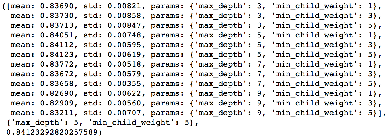
Here, we have run 12 combinations with wider intervals between values. The ideal values are 5 for max_depth and 5 for min_child_weight. Let’s go one step deeper and look for optimum values. We’ll search for values 1 above and below the optimum values because we took an interval of two.
param_test2 = {
 'max_depth':[4,5,6],
 'min_child_weight':[4,5,6]
}
gsearch2 = GridSearchCV(estimator = XGBClassifier( learning_rate=0.1, n_estimators=140, max_depth=5,
 min_child_weight=2, gamma=0, subsample=0.8, colsample_bytree=0.8,
 objective= 'binary:logistic', nthread=4, scale_pos_weight=1,seed=27),
 param_grid = param_test2, scoring='roc_auc',n_jobs=4,iid=False, cv=5)
gsearch2.fit(train[predictors],train[target])
gsearch2.grid_scores_, gsearch2.best_params_, gsearch2.best_score_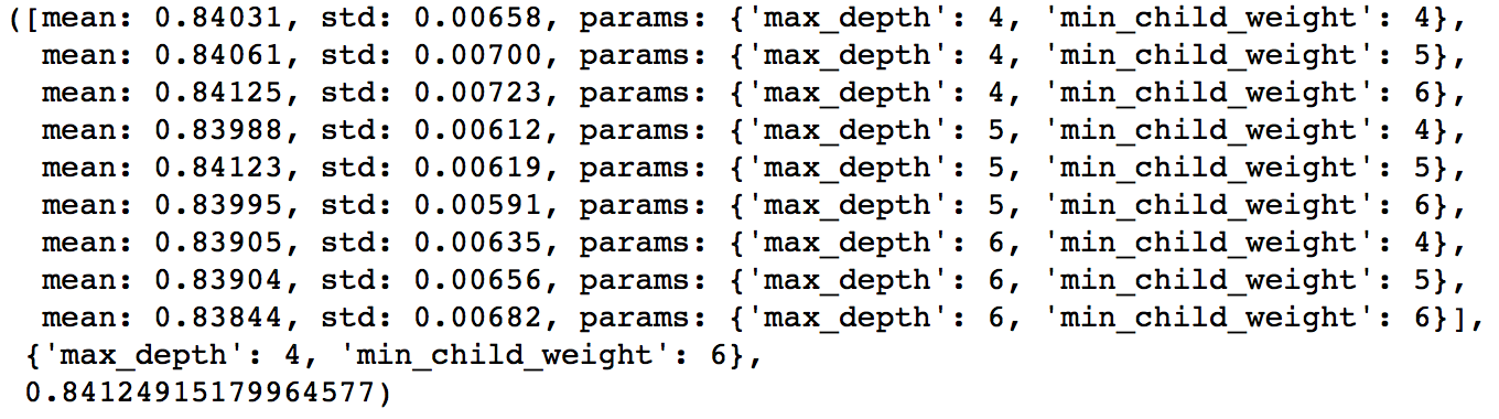
Here, we get the optimum values as 4 for max_depth and 6 for min_child_weight. Also, we can see the CV score increasing slightly. Note that as the model performance increases, it becomes exponentially difficult to achieve even marginal gains in performance. You would have noticed that here we got 6 as the optimum value for min_child_weight, but we haven’t tried values more than 6. We can do that as follow:
param_test2b = {
 'min_child_weight':[6,8,10,12]
}
gsearch2b = GridSearchCV(estimator = XGBClassifier( learning_rate=0.1, n_estimators=140, max_depth=4,
 min_child_weight=2, gamma=0, subsample=0.8, colsample_bytree=0.8,
 objective= 'binary:logistic', nthread=4, scale_pos_weight=1,seed=27),
 param_grid = param_test2b, scoring='roc_auc',n_jobs=4,iid=False, cv=5)
gsearch2b.fit(train[predictors],train[target])
modelfit(gsearch3.best_estimator_, train, predictors)
gsearch2b.grid_scores_, gsearch2b.best_params_, gsearch2b.best_score_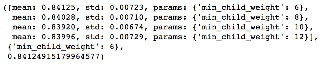
We see 6 as the optimal value.
Step 3: Tune gamma.
Now let’s tune the gamma value using the parameters already tuned above. Gamma can take various values, but I’ll check for 5 values here. You can go into more precise values.
param_test3 = {
 'gamma':[i/10.0 for i in range(0,5)]
}
gsearch3 = GridSearchCV(estimator = XGBClassifier( learning_rate =0.1, n_estimators=140, max_depth=4,
 min_child_weight=6, gamma=0, subsample=0.8, colsample_bytree=0.8,
 objective= 'binary:logistic', nthread=4, scale_pos_weight=1,seed=27),
 param_grid = param_test3, scoring='roc_auc',n_jobs=4,iid=False, cv=5)
gsearch3.fit(train[predictors],train[target])
gsearch3.grid_scores_, gsearch3.best_params_, gsearch3.best_score_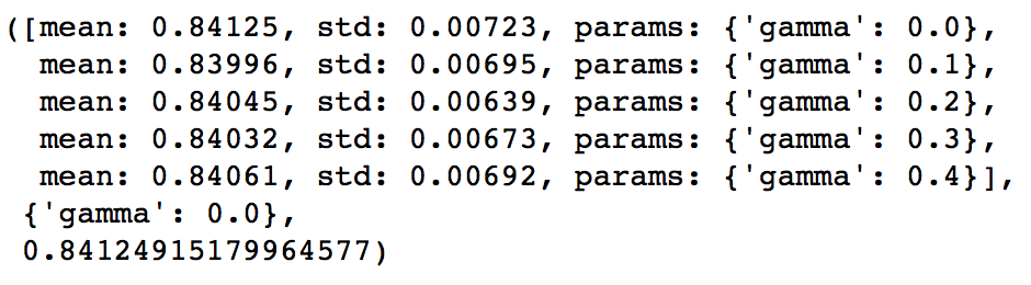
This shows that our original value of gamma, i.e., 0 is the optimum one. Before proceeding, a good idea would be to re-calibrate the number of boosting rounds for the updated parameters.
xgb2 = XGBClassifier(
 learning_rate =0.1,
 n_estimators=1000,
 max_depth=4,
 min_child_weight=6,
 gamma=0,
 subsample=0.8,
 colsample_bytree=0.8,
 objective= 'binary:logistic',
 nthread=4,
 scale_pos_weight=1,
 seed=27)
modelfit(xgb2, train, predictors)
Here, We can see the score improvement. so, the final parameters are:
- max_depth: 4
- min_child_weight: 6
- gamma: 0
Step 4: Tune subsample and colsample_bytree
The next step would be to try different subsample and colsample_bytree values. Let’s do this in 2 stages as well and take values 0.6,0.7,0.8,0.9 for both to start with.
param_test4 = {
 'subsample':[i/10.0 for i in range(6,10)],
 'colsample_bytree':[i/10.0 for i in range(6,10)]
}
gsearch4 = GridSearchCV(estimator = XGBClassifier( learning_rate =0.1, n_estimators=177, max_depth=4,
 min_child_weight=6, gamma=0, subsample=0.8, colsample_bytree=0.8,
 objective= 'binary:logistic', nthread=4, scale_pos_weight=1,seed=27),
 param_grid = param_test4, scoring='roc_auc',n_jobs=4,iid=False, cv=5)
gsearch4.fit(train[predictors],train[target])
gsearch4.grid_scores_, gsearch4.best_params_, gsearch4.best_score_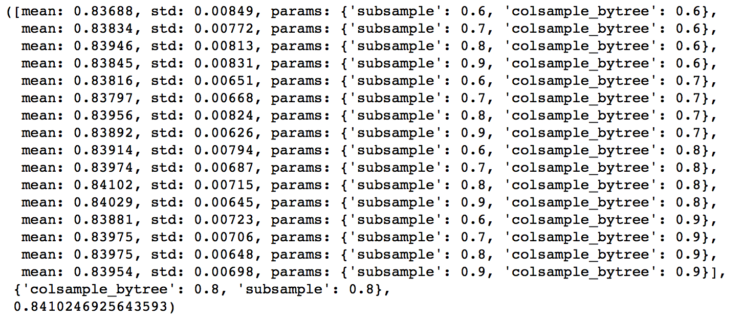
Here, we found 0.8 as the optimum value for both subsample and colsample_bytree. Now we should try values in 0.05 intervals around these.
param_test5 = {
 'subsample':[i/100.0 for i in range(75,90,5)],
 'colsample_bytree':[i/100.0 for i in range(75,90,5)]
}
gsearch5 = GridSearchCV(estimator = XGBClassifier( learning_rate =0.1, n_estimators=177, max_depth=4,
 min_child_weight=6, gamma=0, subsample=0.8, colsample_bytree=0.8,
 objective= 'binary:logistic', nthread=4, scale_pos_weight=1,seed=27),
 param_grid = param_test5, scoring='roc_auc',n_jobs=4,iid=False, cv=5)
gsearch5.fit(train[predictors],train[target])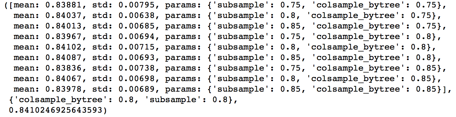
Again we got the same values as before. Thus the optimum values are:
- subsample: 0.8
- colsample_bytree: 0.8
Step 5: Tuning regularization parameters
The next step is to apply regularization to reduce overfitting. However, many people don’t use this parameter much as gamma provides a substantial way of controlling complexity. But we should always try it. I’ll tune the ‘reg_alpha’ value here and leave it up to you to try different values of ‘reg_lambda’.
param_test6 = {
 'reg_alpha':[1e-5, 1e-2, 0.1, 1, 100]
}
gsearch6 = GridSearchCV(estimator = XGBClassifier( learning_rate =0.1, n_estimators=177, max_depth=4,
 min_child_weight=6, gamma=0.1, subsample=0.8, colsample_bytree=0.8,
 objective= 'binary:logistic', nthread=4, scale_pos_weight=1,seed=27),
 param_grid = param_test6, scoring='roc_auc',n_jobs=4,iid=False, cv=5)
gsearch6.fit(train[predictors],train[target])
gsearch6.grid_scores_, gsearch6.best_params_, gsearch6.best_score_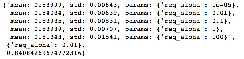
We can see that the CV score is less than in the previous case. But the values tried are very widespread. We should try values closer to the optimum here (0.01) to see if we get something better.
param_test7 = {
 'reg_alpha':[0, 0.001, 0.005, 0.01, 0.05]
}
gsearch7 = GridSearchCV(estimator = XGBClassifier( learning_rate =0.1, n_estimators=177, max_depth=4,
 min_child_weight=6, gamma=0.1, subsample=0.8, colsample_bytree=0.8,
 objective= 'binary:logistic', nthread=4, scale_pos_weight=1,seed=27),
 param_grid = param_test7, scoring='roc_auc',n_jobs=4,iid=False, cv=5)
gsearch7.fit(train[predictors],train[target])
gsearch7.grid_scores_, gsearch7.best_params_, gsearch7.best_score_
You can see that we got a better CV. Now we can apply this regularization in the model and look at the impact:
xgb3 = XGBClassifier(
 learning_rate =0.1,
 n_estimators=1000,
 max_depth=4,
 min_child_weight=6,
 gamma=0,
 subsample=0.8,
 colsample_bytree=0.8,
 reg_alpha=0.005,
 objective= 'binary:logistic',
 nthread=4,
 scale_pos_weight=1,
 seed=27)
modelfit(xgb3, train, predictors)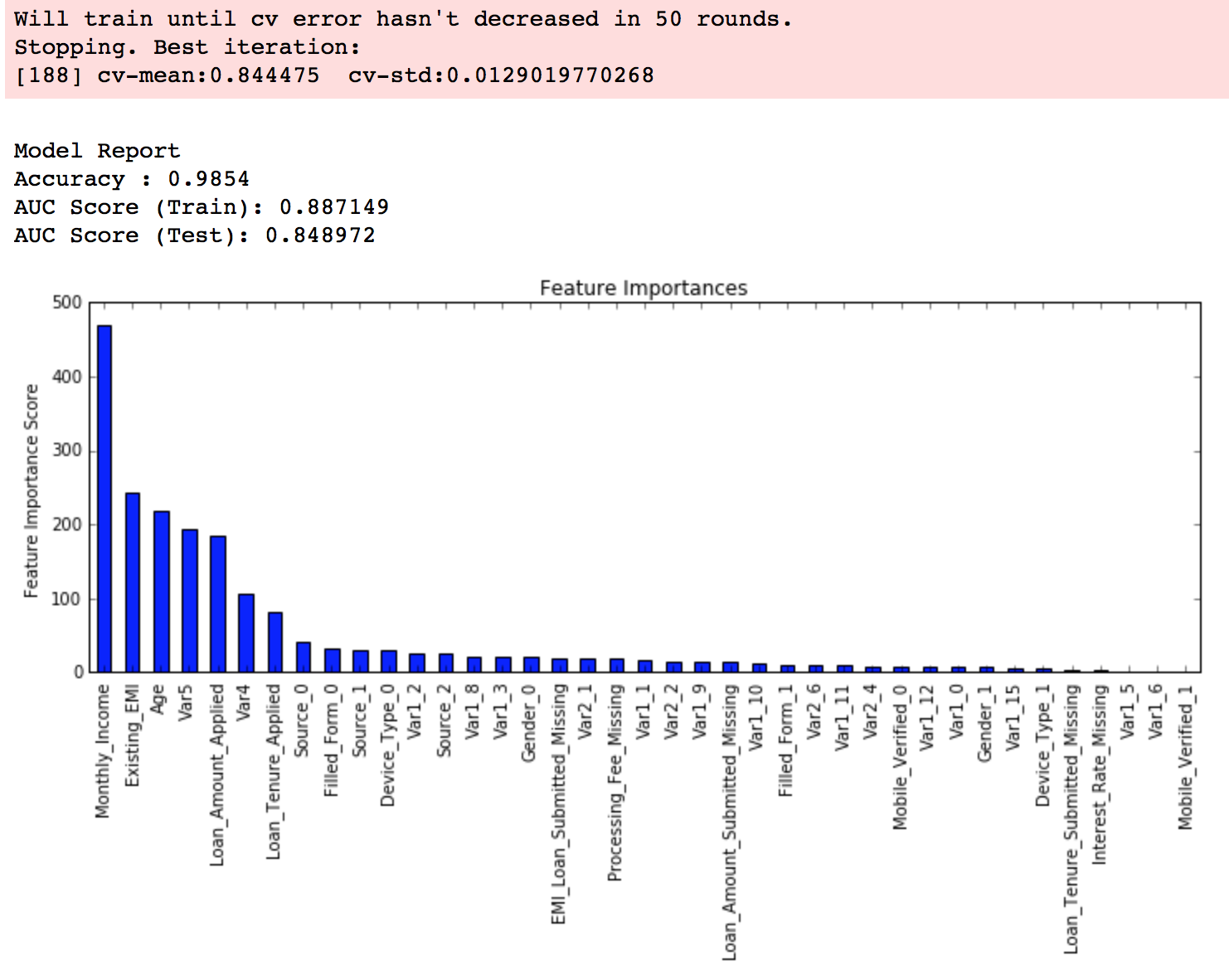
Again we can see a slight improvement in the score.
Step 6: Reducing the learning rate
Lastly, we should lower the learning rate and add more trees. Let’s use the cv function of XGBoost to do the job again.
xgb4 = XGBClassifier(
 learning_rate =0.01,
 n_estimators=5000,
 max_depth=4,
 min_child_weight=6,
 gamma=0,
 subsample=0.8,
 colsample_bytree=0.8,
 reg_alpha=0.005,
 objective= 'binary:logistic',
 nthread=4,
 scale_pos_weight=1,
 seed=27)
modelfit(xgb4, train, predictors)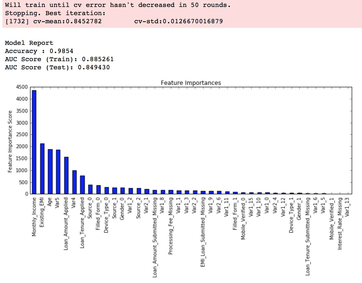
Here is a live coding window where you can try different parameters and test the results.
Now we can see a significant boost in performance, and the effect of parameter tuning is clearer.
As we come to an end, I would like to share 2 key thoughts:
- It is difficult to get a very big leap in performance by just using parameter tuning or slightly better models. The max score for GBM was 0.8487, while XGBoost gave 0.8494. This is a decent improvement but not something very substantial.
- A significant jump can be obtained by other methods like feature engineering, creating an ensemble of models, stacking, etc.
You can also download the iPython notebook with all these model codes from my GitHub account. For codes in R, you can refer to this article.
Master XGBoost Parameters
This tutorial was based on developing an XGBoost machine learning model end-to-end. We started by discussing why XGBoost Parameters has superior performance over GBM, which was followed by a detailed discussion of the various parameters involved. We also defined a generic function that you can reuse for making models. Finally, we discussed the general approach towards tackling a problem with XGBoost and also worked out the AV Data Hackathon 3.x problem through that approach.
Key Takeaways
- XGBoost Paramters is a powerful machine-learning algorithm, especially where speed and accuracy are concerned.
- We need to consider different parameters and their values to be specified while implementing an XGBoost model.
- The XGBoost model requires parameter tuning to improve and fully leverage its advantages over other algorithms.
If you’re looking to take your machine learning skills to the next level, consider enrolling in our Data Science Black Belt program. The curriculum covers all aspects of data science, including advanced topics like XGBoost parameter tuning. With hands-on projects and mentorship, you’ll gain practical experience and the skills you need to succeed in this exciting field. Enroll today and take your XGBoost parameters tuning skills and overall data science expertise to the next level!
Frequently Asked Questions
A. The choice of XGBoost parameters depends on the specific task. Commonly adjusted parameters include learning rate (eta), maximum tree depth (max_depth), and minimum child weight (min_child_weight).
A. The ‘n_estimators’ parameter in XGBoost determines the number of boosting rounds or trees to build. It directly impacts the model’s complexity and should be tuned for optimal performance.
A. In XGBoost, a hyperparameter is a preset setting that isn’t learned from the data but must be configured before training. Examples include the learning rate, tree depth, and regularization parameters.
A. XGBoost provides L1 and L2 regularization terms using the ‘alpha’ and ‘lambda’ parameters, respectively. These parameters prevent overfitting by adding penalty terms to the objective function during training.
Aarshay graduated from MS in Data Science at Columbia University in 2017 and is currently an ML Engineer at Spotify New York. He works at an intersection or applied research and engineering while designing ML solutions to move product metrics in the required direction. He specializes in designing ML system architecture, developing offline models and deploying them in production for both batch and real time prediction use cases.


Please provide the R code as well. Thnkx
It is a great article , but if you could provide codes in R , it would be more beneficial to us. Thanks
Nowadays less people are using R already. Python is the way to go
Hi guys, Thanks for reaching out! I've given a link to an article (http://www.analyticsvidhya.com/blog/2016/01/xgboost-algorithm-easy-steps/) in my above article. This has some R codes for implementing XGBoost in R. This won't replicate the results I found here but will definitely help you. Also, I don't use R much but think it should not be very difficult for someone to code it in R. I encourage you to give it a try and share the code as well if you wish :D. In the meanwhile, I'll also try to get someone to write R codes. I'll get back to you if I find something. Cheers, Aarshay
I am wondering whether in practice it is useful such an extreme tuning of the parameters ... it seems that often the standard deviation on the cross validation folds does not allow to really distinguish between different parameters sets... any thoughts on that?
Agree but partially. Some thoughts: 1. Though the standard deviations are high, as the mean comes down, their individual values should also come down (though theoretically not necessary). Actually the point is that some basic tuning helps but as we go deeper, the gains are just marginal. If you think practically, the gains might not be significant. But when you in a competition, these can have an impact because people are close and many times the difference between winning and loosing is 0.001 or even smaller. 2. As we tune our models, it becomes more robust. Even is the CV increases just marginally, the impact on test set may be higher. I've seen Kaggle master's taking AWS instances for hyper-parameter tuning to test out very small differences in values. 3. I actually look at both mean and std of CV. There are instances where the mean is almost the same but std is lower. You can prefer those models at times. 4. As I mentioned in the end, techniques like feature engineering and blending have a much greater impact than parameter tuning. For instance, I generally do some parameter tuning and then run 10 different models on same parameters but different seeds. Averaging their results generally gives a good boost to the performance of the model. Hope this helps. Please share your thoughts.
Wow this seems to be very interesting I am new to Python and R programming I am really willing to learn this programming. Will be grateful if anyone here can guide me through that what should I learn first or from where should I start. Thanks Jay
Well Jay you have come to the right place! Check out this learning path for Python - http://www.analyticsvidhya.com/learning-paths-data-science-business-analytics-business-intelligence-big-data/learning-path-data-science-python/ You can start with this complete tutorial on python as well - http://www.analyticsvidhya.com/blog/2016/01/complete-tutorial-learn-data-science-python-scratch-2/ You'll find similar resources for R as well here. Along with programming, there are detailed tutorials on data science concepts like this one. You're in for a treat!! Cheers, Aarshay
Hi.. Nice article with lots of informations. I was wondering if I can clear my understandings on following : a) On Handling Missing Values, XGBoost tries different things as it encounters a missing value on each node and learns which path to take for missing values in future. Please elaborate on this. b) In function modelfit; the following has been used xgb_param = alg.get_xgb_params() Is get_xgb_params() available in xgb , what does it passes to xgb_param Please explain: alg.set_params(n_estimators=cvresult.shape[0]) Thanks.
Glad you liked it.. My responses below: a) When xgboost encounters a missing value at a node, it tries both left and right hand split and learns the way leading to higher loss for each node. It then does the same when working on testing data. b) Yes it is available in sklearn wrapper of xgboost package. It will pass the parameters in actual xgboost format (not sklearn wrapper). The cv function requires parameters in that format itself. c) cvresults is a dataframe with the number of rows being equal to the optimum number of parameters selected. You can try printing cvresults and it'll be clear. Hope this helps.
Fantastic work ! thanks a lot. Now let's hope that we will be able to install XGBoost with a simple pip command :)
Thanks :) i think installation is not that simple. depending on the OS, you can refer to different sections of this page - https://github.com/dmlc/xgboost/blob/master/doc/build.md
Hi Guys, I cant seem to predict probabilities, the gbm.predict is only giving me 0's and 1's.. I put objective="binary:logistic" in but I still only get 0 or 1.. Any tips?
sklearn model classes have a function "predict_proba" for predicting the probabilities. Please use that.
During feature engineering, if I want to check if a simple change is producing any effect on performance, should I go through the entire process of fine tuning the parameters, which is obviously better than keeping the same parameter values but takes lot of time. So, how often do you tune your parameters?
Hi Vikas, I don't think that should be required. Once you tune your model on a baseline input, it should be good enough to check if the features are working. If you're experimenting a lot, it might be a good idea to use random forest to check if feature improved the accuracy. RF models run faster and are not much affected by tuning. Hope this helps.
excellent article..... We want Neural Networks as well.
Thanks.. NN is in the pipeline.. :)
At section 3 : - 3.Parameter With tuning, xgtest = xgb.DMatrix(dtest[predictors].values) dtest doesnt exist. Where did you get it? Im trying to learn with your code! Thanks in advance
Hi Andre, Thanks for reaching out. Valid point. My bad I should have removed it. I've updated the code above. The reason it was present is that I used the test file on my end for checking the result of each model, which can be seen as "AUC Score (Test)". You would not get this output when you run it locally on your system. Hope this clears the confusion.
Hi Jain thanks for you effort, this guide is simply awesome ! But just because I wasn't able to find the modified Train Data from the repository (in effect I wasn't able to find the repository, my fault for sure, but I'm working on it), I had to rebuild the modified train data (good exercise !) and I want to share with everyone my code: train.ix[ train['DOB'].isnull(), 'DOB' ] = train['DOB'].max() train['Age'] = (pd.to_datetime( train['DOB'].max(), dayfirst=True ) - pd.to_datetime( train['DOB'], dayfirst=True )).astype('int64') train.ix[ train['EMI_Loan_Submitted'].isnull(), 'EMI_Loan_Submitted_Missing' ] = 1 train.ix[ train['EMI_Loan_Submitted'].notnull(), 'EMI_Loan_Submitted_Missing' ] = 0 train.ix[ train['Existing_EMI'].isnull(), 'Existing_EMI' ] = train['Existing_EMI'].median() train.ix[ train['Interest_Rate'].isnull(), 'Interest_Rate_Missing' ] = 1 train.ix[ train['Interest_Rate'].notnull(), 'Interest_Rate_Missing' ] = 0 train.ix[ train['Loan_Amount_Applied'].isnull(), 'Loan_Amount_Applied' ] = train['Loan_Amount_Applied'].median() train.ix[ train['Loan_Tenure_Applied'].isnull(), 'Loan_Tenure_Applied' ] = train['Loan_Tenure_Applied'].median() train.ix[ train['Loan_Amount_Submitted'].isnull(), 'Loan_Amount_Submitted_Missing' ] = 1 train.ix[ train['Loan_Amount_Submitted'].notnull(), 'Loan_Amount_Submitted_Missing' ] = 0 train.ix[ train['Loan_Tenure_Submitted'].isnull(), 'Loan_Tenure_Submitted_Missing' ] = 1 train.ix[ train['Loan_Tenure_Submitted'].notnull(), 'Loan_Tenure_Submitted_Missing' ] = 0 train.ix[ train['Processing_Fee'].isnull(), 'Processing_Fee_Missing' ] = 1 train.ix[ train['Processing_Fee'].notnull(), 'Processing_Fee_Missing' ] = 0 train.ix[ ( train['Source'] != train['Source'].value_counts().index[0] ) & ( train['Source'] != train['Source'].value_counts().index[1] ), 'Source' ] = 'S000' # Numerical Categorization from sklearn.preprocessing import LabelEncoder var_mod = [] # Nessun valore numerico da categorizzare, in caso contrario avremmo avuto una lista di colonne le = LabelEncoder() for i in var_mod: train[i] = le.fit_transform(train[i]) #One Hot Coding: train = pd.get_dummies(train, columns=['Source', 'Gender', 'Mobile_Verified', 'Filled_Form', 'Device_Type','Var1','Var2']) train.drop(['City','DOB','EMI_Loan_Submitted','Employer_Name','Interest_Rate','Lead_Creation_Date','Loan_Amount_Submitted', 'Loan_Tenure_Submitted','LoggedIn','Salary_Account','Processing_Fee'], axis=1, inplace=True) Just because the way I constructed my "age" column, results are a little different, but plus or minus all ought to be right. Thanks everyone, this site is pure gold for me. I learned here in a month more than I learned everywhere in years ... I'm just guessing where I will be in a year from now.
Hi Gianni, Thanks for your effort and for sharing the code. The data set has been uploaded and a link provided inside the article at section 3. Parameter Tuning with Example line 3. You can also download the same from my GitHub repository: https://github.com/aarshayj/Analytics_Vidhya/tree/master/Articles/Parameter_Tuning_XGBoost_with_Example The filename is 'train_modified.zip' Cheers, Aarshay
Guys, Please help me with xgboost installation on windows
I use a MAC OS so I haven't tried on windows. I think installing on R is pretty straight forward but Python is a challenge. I guess the discussion forum is the right place to reach out to a wider audience who can help. :)
I followed instructions from the below link and it worked for me http://stackoverflow.com/a/35119904 Long story short, I have installed "mingw64" and "Cygwin shell" on my laptop and ran the commands provided in the above answer.
I have the error cvresult = xgb.cv(xgb_param, xgtrain, num_boost_round=alg.get_params()['n_estimators'], nfold=cv_folds, metrics='auc', early_stopping_rounds=early_stopping_rounds, show_progress=False) raise ValueError('Check your params.'\ ValueError: Check your params.Early stopping works with single eval metric only. How can I fix it? Thank you in advance.
What I can understand from the error is that multiple metrics have been defined. But here it's just 'auc'. Please check your xgb_param value. Is it setting a different value for metric? If problem persists for long, I suggest you start a discussion thread with code and error snapshot. It'll be easier to debug.
Hi Aarshay, quick question: if I try to do multi-class classification, python send error as follows: xgb1 = XGBClassifier( learning_rate =0.1, n_estimators=1000, max_depth=5, min_child_weight=1, gamma=0, subsample=0.8, colsample_bytree=0.8, n_class=4, objective="multi:softmax", nthread=4, scale_pos_weight=1, seed=27) Traceback (most recent call last): File "", line 15, in seed=27) TypeError: __init__() got an unexpected keyword argument 'n_class' When i try "num_class" instead it does not work either nor with "n_classes" the sklearn wrapper I assume, Any Thoughts? thanks, Daniel
Hi Daniel, I don't think the 'n_classes' or any other variant of argument is needed in the sklearn wrapper. It works for me without this argument. Please try removing it.
Hi Daniel, I met the same problem as you. Can not figure out how to add "num_class" parameter to XGBClassifer(). If you figure it out, could you please show us how to solve this problem? Thanks a lot! Michelle
Hi Aarshay, The youtube video link you posted is not working. (Error is "This video is private") https://www.youtube.com/watch?v=X47SGnTMZIU Is there any other source where we can watch the video? Thanks, Praveen
try this - https://www.youtube.com/watch?v=ufHo8vbk6g4
Hi Praveen, I followed the steps to install XGB on Windows 7 as mentioned in your comment above i.e using mingw64 and cygwin/ Everything went fine until the last steps as below: cp make/mingw64.mk config.mk make -j4 --->>> where (make = mingw32-make) By running the above lines I get the error as follows:: g++ -m64 -std=c++0x -Wall -O3 -msse2 -Wno-unknown-pragmas -funroll-loops -Iincl ude -DDMLC_ENABLE_STD_THREAD=0 -Idmlc-core/include -Irabit/include -fopenmp -MM -MT build/logging.o src/logging.cc >build/logging.d g++ -m64 -std=c++0x -Wall -O3 -msse2 -Wno-unknown-pragmas -funroll-loops -Iincl ude -DDMLC_ENABLE_STD_THREAD=0 -Idmlc-core/include -Irabit/include -fopenmp -MM -MT build/learner.o src/learner.cc >build/learner.d g++ -m64 -std=c++0x -Wall -O3 -msse2 -Wno-unknown-pragmas -funroll-loops -Iincl ude -DDMLC_ENABLE_STD_THREAD=0 -Idmlc-core/include -Irabit/include -fopenmp -MM -MT build/c_api/c_api.o src/c_api/c_api.cc >build/c_api/c_api.d g++ -m64 -std=c++0x -Wall -O3 -msse2 -Wno-unknown-pragmas -funroll-loops -Iincl ude -DDMLC_ENABLE_STD_THREAD=0 -Idmlc-core/include -Irabit/include -fopenmp -MM -MT build/data/simple_dmatrix.o src/data/simple_dmatrix.cc >build/data/simple_d matrix.d g++ -m64 -c -std=c++0x -Wall -O3 -msse2 -Wno-unknown-pragmas -funroll-loops -Iinclude -DDMLC_ENABLE_STD_THREAD=0 -Idmlc-core/include -Irabit/include -fopenmp -c src/logging.cc -o build/logging.o g++ -m64 -c -std=c++0x -Wall -O3 -msse2 -Wno-unknown-pragmas -funroll-loops -Iinclude -DDMLC_ENABLE_STD_THREAD=0 -Idmlc-core/include -Irabit/include -fopenmp -c src/c_api/c_api.cc -o build/c_api/c_api.o g++ -m64 -c -std=c++0x -Wall -O3 -msse2 -Wno-unknown-pragmas -funroll-loops -Iinclude -DDMLC_ENABLE_STD_THREAD=0 -Idmlc-core/include -Irabit/include -fopenmp -c src/data/simple_dmatrix.cc -o build/data/simple_dmatrix.o In file included from include/xgboost/./base.h:10:0, from include/xgboost/logging.h:13, from src/logging.cc:7: dmlc-core/include/dmlc/omp.h:9:17: fatal error: omp.h: No such file or directory compilation terminated. g++ -m64 -c -std=c++0x -Wall -O3 -msse2 -Wno-unknown-pragmas -funroll-loops -Iinclude -DDMLC_ENABLE_STD_THREAD=0 -Idmlc-core/include -Irabit/include -fopenmp -c src/learner.cc -o build/learner.o Makefile:97: recipe for target 'build/logging.o' failed make: *** [build/logging.o] Error 1 make: *** Waiting for unfinished jobs.... In file included from include/xgboost/./base.h:10:0, from include/xgboost/logging.h:13, from src/learner.cc:7: dmlc-core/include/dmlc/omp.h:9:17: fatal error: omp.h: No such file or directory compilation terminated. Makefile:97: recipe for target 'build/learner.o' failed make: *** [build/learner.o] Error 1 In file included from include/xgboost/./base.h:10:0, from include/xgboost/data.h:15, from src/data/simple_dmatrix.cc:7: dmlc-core/include/dmlc/omp.h:9:17: fatal error: omp.h: No such file or directory compilation terminated. Makefile:97: recipe for target 'build/data/simple_dmatrix.o' failed make: *** [build/data/simple_dmatrix.o] Error 1 In file included from include/xgboost/./base.h:10:0, from include/xgboost/data.h:15, from src/c_api/c_api.cc:3: dmlc-core/include/dmlc/omp.h:9:17: fatal error: omp.h: No such file or directory compilation terminated. Makefile:97: recipe for target 'build/c_api/c_api.o' failed make: *** [build/c_api/c_api.o] Error 1 I don't understand the reason behind this error. I have stored the mingw64 files under C:\mingw64\mingw64 And I have stored the xgboost files under C:\xgboost. I also added the paths to Environment.as well. I even tried to install the same way in my oracle virtual box but it threw the same building error there too. Please could you throw some light on this and let me know if I am missing anything ??
Hi Aarshay, As always, a great article. I have two doubts 1. n_estimators=cvresult.shape[0] we have set this while fitting the algorithm for XGBoost. Any specific reason why we did in that way. 2. In the model fit function, we are not generating CV score as the output.. How are we automatically able to get it in box with red background. I am not getting CV value. Am I missing something? Can you please clarify Regards, Praveen
Hi..Praveen Gupta Sanka, Can you please share how to install xgboost in python/ anaconda env. ? r I followed instructions from the below link and it worked for me http://stackoverflow.com/a/35119904 Can you please share how you installed “mingw64” and “Cygwin shell” on laptop ? Need hand holding on the same. Thanks in advance,
Thanks Praveen! My responses: 1. I've used xgb.cv here for determining the optimum number of estimators for a given learning rate. After running xgb.cv, this statement overwrites the default number of estimators to that obtained from xgb.cv. The variable cvresults is a dataframe with as many rows as the number of final estimators. 2. The red box is also a result of the xgb.cv function call.
When I try the GridSearchCV my system does not do anything. It sits there for a long time, but I can check the activity monitor and nothing happens, no crash, no message, no activity. Any clue?
This is strange indeed. Right off the bat, I think of following diagnosis: 1. Run the GridSearchCV for a very small sample of data, the one which you are sure your system can handle easily. This will check the installation of sklearn 2. If it works fine, it might be a system computing power issue. If it doesn't work try re-installing sklearn.
I get an error: XGBClassifier' object has no attribute 'feature_importances_' It looks like it a known issue with XGBClassifier. See https://www.kaggle.com/c/homesite-quote-conversion/forums/t/18669/xgb-importance-question-lost-features-advice/106421 and https://github.com/dmlc/xgboost/issues/757#issuecomment-174550974 I can get the feature importances with the following: def importance_XGB(clf): impdf = [] for ft, score in clf.booster().get_fscore().iteritems(): impdf.append({'feature': ft, 'importance': score}) impdf = pd.DataFrame(impdf) impdf = impdf.sort_values(by='importance', ascending=False).reset_index(drop=True) impdf['importance'] /= impdf['importance'].sum() return impdf importance_XGB(xgb1)
I actually got it working by updating to the latest version of XGBoost. However, I had to change metrics='auc' to metrics={'auc'} Also, early_stopping_rounds does not appear to work anymore
Sorry to bother you again, but would you mind elaborating a little more on the code in modelfit, in particular: if useTrainCV: xgb_param = alg.get_xgb_params() xgtrain = xgb.DMatrix(dtrain[predictors].values, label=dtrain[target].values) cvresult = xgb.cv(xgb_param, xgtrain, num_boost_round=alg.get_params()['n_estimators'], nfold=cv_folds, metrics='auc', early_stopping_rounds=early_stopping_rounds, show_progress=False) alg.set_params(n_estimators=cvresult.shape[0]) Thank you very for your time.
sure. this part of the code would check the optimal number of estimators using the "cv" function of xgboost. This works only if the useTrainCV argument of the function is set as True. If True, this will run "xgb.cv", determine the optimal value for n_estimators and replace the value set by the user with this value. While using this case, you should remember to set a very high value for n_estimators, i.e. higher than the expected optimal value range. Hope this makes sense.
Thanks for your work here - great job! Is it be possible to be notified when a similar article to this one is released for Neural Networks?
They are already out there: 1. http://www.analyticsvidhya.com/blog/2016/03/introduction-deep-learning-fundamentals-neural-networks/ 2. http://www.analyticsvidhya.com/blog/2016/04/deep-learning-computer-vision-introduction-convolution-neural-networks/
Hello, really great article, I have learnt a lot from it. One question, you mention the default value for scale_pos_weight is 0. Where have you got this information from? Checking the source code (regresion_obj.cc) I have found the value to be 1 by default, with a lower bound of 0. In the R version, that I use, the parameter does not appear explicitly. Can you please clarify? Thanks in advance
I just checked again. Yes you're right the default value is 1 and not 0. Thanks for pointing this out. I'll make the correction.
I'm getting this strange error:"WindowsError: exception: access violation reading 0x000000000D92066C" Any Idea what may be causing it? FYI, if I don't include the [] on the metric parameter, I get: "ValueError: Check your params.Early stopping works with single eval metric only." (same as the user above) cvresult = xgb.cv(xgb_param, xgtrain, num_boost_round=alg.get_params()['n_estimators'], nfold=5, metrics=['logloss'], early_stopping_rounds=25, show_progress=False) Will train until cv error hasn't decreased in 25 rounds. Traceback (most recent call last): File "", line 2, in metrics=['logloss'], early_stopping_rounds=25, show_progress=False) File "C:\Anaconda2\lib\site-packages\xgboost-0.4-py2.7.egg\xgboost\training.py", line 415, in cv cvfolds = mknfold(dtrain, nfold, params, seed, metrics, fpreproc) File "C:\Anaconda2\lib\site-packages\xgboost-0.4-py2.7.egg\xgboost\training.py", line 275, in mknfold dtrain = dall.slice(np.concatenate([idset[i] for i in range(nfold) if k != i])) File "C:\Anaconda2\lib\site-packages\xgboost-0.4-py2.7.egg\xgboost\core.py", line 494, in slice ctypes.byref(res.handle))) WindowsError: exception: access violation reading 0x000000000D92066C
not sure man. have you tried searching? posting on discussion forum might be a good idea to crowd-source the issue.
According to this: https://www.kaggle.com/c/santander-customer-satisfaction/forums/t/20662/overtuning-hyper-parameters-especially-re-xgboost If you are using logistic trees, as I understand your article describes, alpha and lambda don't play any role. I would appreciate your feedback Thanks in advance
Hi Jose, I'm not sure which part of the post you are referring to. If it is the part which says "reg_alpha, reg_lambda are not used in tree booster", then this is right. But the parameters which I've mentioned are alpha and lambda and not reg_alpha and reg_lambda. Regularization is used in tree-booster as well where the constraint is put on the score of each leaf in the tree. Please let me know if its still unclear. Cheers!
It is a great blog. It will be better, if you can give a parameter tuning for a regression problem, although a lot of stuff will be similiar to the classification problem.
Yes its mostly similar. If you understand this, the regression part should be easy to manage.
Thanks great article.
Great article. Thank you.
Thanks for the article, very useful :-) I was wondering if an article on "stacking" was in the pipe?
Hi Jian, Just a quick question. you use test_results.csv in modelfit function. Where is the cvs file? I couldn't find it. test_results = pd.read_csv('test_results.csv') Thank you. Michelle
[…] I explain how to enable multi threading for XGBoost, let me point you to this excellent Complete Guide to Parameter Tuning in XGBoost (with codes in Python). I found it useful as I started using XGBoost. And I assume that you could be interested if you […]
[…] I explain how to enable multi threading for XGBoost, let me point you to this excellent Complete Guide to Parameter Tuning in XGBoost (with codes in Python). I found it useful as I started using XGBoost. And I assume that you could be interested if you […]
1) Hi can you also share how to use a new dataset to be predicted upon completing the above mentioned tuning processes. 2)Also by ensembles of model, if I'm right does it mean like I use multiple models to classify / predict and finally use the predictions as features and create a model on top of it?
Hi, Thanks for sharing. One question: how do you decide what random seed to use. Is 27 just a random pick?
Hi guys, Is there anyone who can run all the code above without getting errors? I got errors in step one and two. It said "ValueError: could not convert string to float: 'S122'" in step 1 and "Parameter values for parameter (max_depth) need to be a sequence" in step two.
This is a great article, Aarshay. Thank you so much for writing it. I am a newbie in data science. Once I follow this article and tune my parameters, how do I get the model to make a prediction on test data and see the prediction? Please help me with sample code. Thank you in advance.
I have one question related to #Predict training set part: One line before this part, we trained the algorithm on the training set. Could you please explain why do we need to find the prediction of the algorithm on the same training set? Regards, Kalle
How can I set tree_method to be 'exact' in XGBoost Classifier? (required for huge datasets)
I ran the code for n_estimator tuning. It showed me the accuracy but didn't show the optimized no. of estimators. What can be the error?
This article is very well done and a helpful guide to get up and running with XGBoost parameter tuning. Once concern I have: Is there a reason why you don't hold out test data or use any type of cross validation for evaluating model performance? Maybe I missed something (I've been known to speed read and skip over important information).
Hi guyz , awesome blog , I had a doubt why is the n_estimator having different values in different steps in step -3 it is = 1000 above it is taken as 140 and the nxt step has 177 at last we have 5000 .
Hello Aarshay This is really great article, I have learnt a lot from it. One question, when i tuning the model using dataset ( size = 1gb ), the model ran very slowly , do you know why it ran too slowly ? Thanks
Thanks Aarshay. This is a great article I am getting an error while trying to make predictions on test data set. Would it be possible to provide a sample code Thanks,
Very impressive, I learned a lot. thanks for writing this! JR
Hi Johan, Thank you for the feedback!
Hi Aarshay! I'm running your code on my own data. For this I use the xgbregressor with objective (reg:linear). I want it to minimize the root mean squared error (RMSE). To do this, I use the neg_mean_squared_error as scoring function in the GridSearchCV. However, in the second part of the tuning (gsearch2 in your code) it gives me best_params_ that result in a lower RMSE. How is this possible? Moreover, the gsearch2.best_score_ gives me values like -77, while the RMSE of this function is 4,413. What should I do to make these two scores agree? Should I change the scoring function? if so, to what should I change it? Cheers
I am not receiving this message box from the first step - there is a pink box with the message before the print output: "Will train until cv error hasn't decreased in 50 rounds. Stopping Best Iteration: [140] : ---" What should I do to have it showing?
hi , Sorry. I did see where is the code to get "140 as the optimal estimators". Could anyone highlight the code to me? Thanks, Sam
If you use too many hyperparameters you will end up overfitting some of them just by chance, even if you use cross-validation.
This is a great article, Aarshay. Thank you so much for writing it. I am a newbie in data science. Once I follow this article and tune my parameters, how do I get the model to make a prediction on test data and see the prediction? Please help me with sample code Parameter Tuning in XGBoost by SPO,GA in python . Thank you in advance.