Introduction
In my last article, I discussed the fundamentals of deep learning, where I explained the basic working of a artificial neural network. If you’ve been following this series, today we’ll become familiar with practical process of implementing neural network in Python (using Theano package).
I found various other packages also such as Caffe, Torch, TensorFlow etc to do this job. But, Theano is no less than and satisfactorily execute all the tasks. Also, it has multiple benefits which further enhances the coding experience in Python.
In this article, I’ll provide a comprehensive practical guide to implement Neural Networks using Theano. If you are here for just python codes, feel free to skip the sections and learn at your pace. And, if you are new to Theano, I suggest you to follow the article sequentially to gain complete knowledge.
Note:
- This article is best suited for users with knowledge of neural network & deep learning.
- If you don’t know python, start here.
- If you don’t know deep learning, start here.

Table of Contents
- Theano Overview
- Implementing Simple expressions
- Theano Variable Types
- Theano Functions
- Modeling a Single Neuron
- Modeling a Two-Layer Networks
1. Theano Overview
In short, we can define Theano as:
- A programming language which runs on top of Python but has its own data structure which are tightly integrated with numpy
- A linear algebra compiler with defined C-codes at the backend
- A python package allowing faster implementation of mathematical expressions
As popularly known, Theano was developed at the University of Montreal in 2008. It is used for defining and evaluating mathematical expressions in general.
Theano has several features which optimize the processing time of expressions. For instance it modifies the symbolic expressions we define before converting them to C codes. Examples:
- It makes the expressions faster, for instance it will change { (x+y) + (x+y) } to { 2*(x+y) }
- It makes expressions more stable, for instance it will change { exp(a) / exp(a).sum(axis=1) } to { softmax(a) }
Below are some powerful advantages of using Theano:
- It defines C-codes for different mathematical expressions.
- The implementations are much faster as compared to some of the python’s default implementations.
- Due to fast implementations, it works well in case of high dimensionality problems.
- It allows GPU implementation which works blazingly fast specially for problems like deep learning.
Let’s now focus on Theano (with example) and try to understand it as a programming language.
2. Implementing Simple Expressions
Lets start by implementing a simple mathematical expression, say a multiplication in Theano and see how the system works. In later sections, we will take a deep dive into individual components. The general structure of a Theano code works in 3 steps:
- Define variables/objects
- Define a mathematical expression in the form of a function
- Evaluate expressions by passing values
Lets look at the following code for simply multiplying 2 numbers:
Step 0: Import libraries
import numpy as np
import theano.tensor as T
from theano import function
Here, we have simply imported 2 key functions of theano – tensor and function.
Step 1: Define variables
a = T.dscalar('a')
b = T.dscalar('b')
Here 2 variables are defined. Note that we have used Theano tensor object type here. Also, the arguments passed to dscalar function are just name of tensors which are useful while debugging. They code will work even without them.
Step 2: Define expression
c = a*b
f = function([a,b],c)
Here we have defined a function f which has 2 arguments:
- Inputs [a,b]: these are inputs to system
- Output c: this has been previously defined
Step 3: Evaluate Expression
f(1.5,3)
![]()
Now we are simply calling the function with the 2 inputs and we get the output as a multiple of the two. In short, we saw how we can define mathematical expressions in Theano and evaluate them. Before we go into complex functions, lets understand some inherent properties of Theano which will be useful in building neural networks.
3. Theano Variable Types
Variables are key building blocks of any programming language. In Theano, the objects are defined as tensors. A tensor can be understood as a generalized form of a vector with dimension t. Different dimensions are analogous to different types:
- t = 0: scalar
- t = 1: vector
- t = 2: matrix
- and so on..
Watch this interesting video to get a deeper level of intuition into vectors and tensors.
These variables can be defined similar to our definition of ‘dscalar’ in the above code. The various keywords for defining variables are:
- byte: bscalar, bvector, bmatrix, brow, bcol, btensor3, btensor4
- 16-bit integers: wscalar, wvector, wmatrix, wrow, wcol, wtensor3, wtensor4
- 32-bit integers: iscalar, ivector, imatrix, irow, icol, itensor3, itensor4
- 64-bit integers: lscalar, lvector, lmatrix, lrow, lcol, ltensor3, ltensor4
- float: fscalar, fvector, fmatrix, frow, fcol, ftensor3, ftensor4
- double: dscalar, dvector, dmatrix, drow, dcol, dtensor3, dtensor4
- complex: cscalar, cvector, cmatrix, crow, ccol, ctensor3, ctensor4
Now you understand that we can define variables with different memory allocations and dimensions. But this is not an exhaustive list. We can define dimensions higher than 4 using a generic TensorType class. You’ll find more details here.
Please note that variables of these types are just symbols. They don’t have a fixed value and are passed into functions as symbols. They only take values when a function is called. But, we often need variables which are constants and which we need not pass in all the functions. For this Theano provides shared variables. These have a fixed value and are not of the types discussed above. They can be defined as numpy data types or simple constants.
Lets take an example. Suppose, we initialize a shared variable as 0 and use a function which:
- takes an input
- adds the input to the shared variable
- returns the square of shared variable
This can be done as:
from theano import shared
x = T.iscalar('x')
sh = shared(0)
f = function([x], sh**2, updates=[(sh,sh+x)])
Note that here function has an additional argument called updates. It has to be a list of lists or tuples, each containing 2 elements of form (shared_variable, updated_value). The output for 3 subsequent runs is:
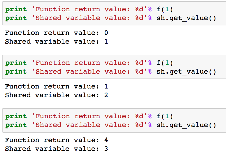
You can see that for each run, it returns the square of the present value, i.e. the value before updating. After the run, the value of shared variable gets updated. Also, note that shared variables have 2 functions “get_value()” and “set_value()” which are used to read and modify the value of shared variables.
4. Theano Functions
Till now we saw the basic structure of a function and how it handles shared variables. Lets move forward and discuss couple more things we can do with functions:
Return Multiple Values
We can return multiple values from a function. This can be easily done as shown in following example:
a = T.dscalar('a')
f = function([a],[a**2, a**3])
f(3)
![]()
We can see that the output is an array with the square and cube of the number passed into the function.
Computing Gradients
Gradient computation is one of the most important part of training a deep learning model. This can be done easily in Theano. Let’s define a function as the cube of a variable and determine its gradient.
x = T.dscalar('x')
y = x**3
qy = T.grad(y,x)
f = function([x],qy)
f(4)
This returns 48 which is 3x2 for x=4. Lets see how Theano has implemented this derivative using the pretty-print feature as following:
from theano import pp  #pretty-print
print(pp(qy))
![]()
In short, it can be explained as: fill(x3,1)*3*x3-1 You can see that this is exactly the derivative of x3. Note that fill(x3,1) simply means to make a matrix of same shape as x3 and fill it with 1. This is used to handle high dimensionality input and can be ignored in this case.
We can use Theano to compute Jacobian and Hessian matrices as well which you can find here.
There are various other aspects of Theano like conditional and looping constructs. You can go into further detail using following resources:
5. Modeling a Single Neuron
Lets start by modeling a single neuron.
Note that I will take examples from my previous article on neuron networks here. If you wish to go in the detail of how these work, please read this article. For modeling a neuron, lets adopt a 2 stage process:
- Implement Feed Forward Pass
- take inputs and determine output
- use the fixed weights for this case
- Implement Backward Propagation
- calculate error and gradients
- update weights using gradients
Lets implement an AND gate for this purpose.
Feed Forward Pass
An AND gate can be implemented as:
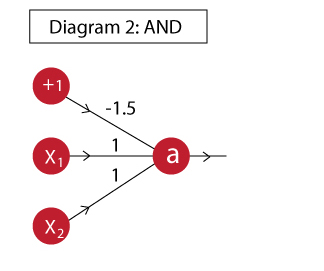
Now we will define a feed forward network which takes inputs and uses the shown weights to determine the output. First we will define a neuron which computes the output a.
import theano
import theano.tensor as T
from theano.ifelse import ifelse
import numpy as np

#Define variables:
x = T.vector('x')
w = T.vector('w')
b = T.scalar('b')

#Define mathematical expression:
z = T.dot(x,w)+b
a = ifelse(T.lt(z,0),0,1)

neuron = theano.function([x,w,b],a)
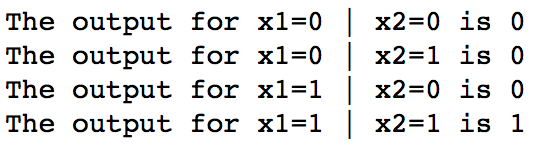
I have simply used the steps we saw above. If you are not sure how this expression works, please refer to the neural networks article I have referred above. Now let’s test out all values in the truth table and see if the AND function has been implemented as desired.
#Define inputs and weights
inputs = [
    [0, 0],
    [0, 1],
    [1, 0],
    [1, 1]
]
weights = [ 1, 1]
bias = -1.5

#Iterate through all inputs and find outputs:
for i in range(len(inputs)):
    t = inputs[i]
    out = neuron(t,weights,bias)
    print 'The output for x1=%d | x2=%d is %d' % (t[0],t[1],out)
Note that, in this case we had to provide weights while calling the function. However, we will be required to update them while training. So, its better that we define them as a shared variable. The following code implements w as a shared variable. Try this out and you’ll get the same output.
import theano
import theano.tensor as T
from theano.ifelse import ifelse
import numpy as np

#Define variables:
x = T.vector('x')
w = theano.shared(np.array([1,1]))
b = theano.shared(-1.5)

#Define mathematical expression:
z = T.dot(x,w)+b
a = ifelse(T.lt(z,0),0,1)

neuron = theano.function([x],a)

#Define inputs and weights
inputs = [
    [0, 0],
    [0, 1],
    [1, 0],
    [1, 1]
]

#Iterate through all inputs and find outputs:
for i in range(len(inputs)):
    t = inputs[i]
    out = neuron(t)
    print 'The output for x1=%d | x2=%d is %d' % (t[0],t[1],out)
Now the feedforward step is complete.
Backward Propagation
Now we have to modify the above code and perform following additional steps:
- Determine the cost or error based on true output
- Determine gradient of node
- Update the weights using this gradient
Lets initialize the network as follow:
#Gradient
import theano
import theano.tensor as T
from theano.ifelse import ifelse
import numpy as np
from random import random

#Define variables:
x = T.matrix('x')
w = theano.shared(np.array([random(),random()]))
b = theano.shared(1.)
learning_rate = 0.01

#Define mathematical expression:
z = T.dot(x,w)+b
a = 1/(1+T.exp(-z))
Note that, you will notice a change here as compared to above program. I have defined x as a matrix here and not a vector. This is more of a vectorized approach where we will determine all the outputs together and find the total cost which is required for determining the gradients.
You should also keep in mind that I am using the full-batch gradient descent here, i.e. we will use all training observations to update the weights.
Let’s determine the cost as follows:
a_hat = T.vector('a_hat') #Actual output
cost = -(a_hat*T.log(a) + (1-a_hat)*T.log(1-a)).sum()
In this code, we have defined a_hat as the actual observations. Then we determine the cost using a simple logistic cost function since this is a classification problem. Now lets compute the gradients and define a means to update the weights.
dw,db = T.grad(cost,[w,b])

train = function(
    inputs = [x,a_hat],
    outputs = [a,cost],
    updates = [
        [w, w-learning_rate*dw],
        [b, b-learning_rate*db]
    ]
)
In here, we are first computing gradient of the cost w.r.t. the weights for inputs and bias unit. Then, the train function here does the weight update job. This is an elegant but tricky approach where the weights have been defined as shared variables and the updates argument of the function is used to update them every time a set of values are passed through the model.
#Define inputs and weights
inputs = [
    [0, 0],
    [0, 1],
    [1, 0],
    [1, 1]
]
outputs = [0,0,0,1]

#Iterate through all inputs and find outputs:
cost = []
for iteration in range(30000):
    pred, cost_iter = train(inputs, outputs)
    cost.append(cost_iter)

#Print the outputs:
print 'The outputs of the NN are:'
for i in range(len(inputs)):
    print 'The output for x1=%d | x2=%d is %.2f' % (inputs[i][0],inputs[i][1],pred[i])

#Plot the flow of cost:
print '\nThe flow of cost during model run is as following:'
import matplotlib.pyplot as plt
%matplotlib inline
plt.plot(cost)
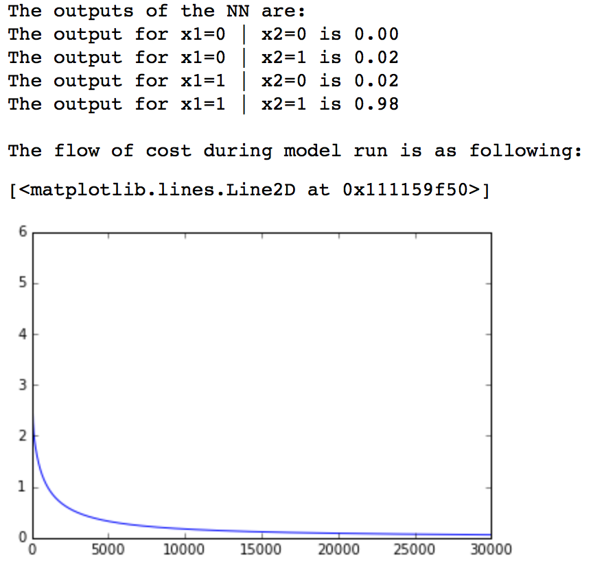
Here we have simply defined the inputs, outputs and trained the model. While training, we have also recorded the cost and its plot shows that our cost reduced towards zero and then finally saturated at a low value. The output of the network also matched the desired output closely. Hence, we have successfully implemented and trained a single neuron.
6. Modeling a Two-Layer Neural Network
I hope you have understood the last section. If not, please do read it multiple times and proceed to this section. Along with learning Theano, this will enhance your understanding of neural networks on the whole.
Lets consolidate our understanding by taking a 2-layer example. To keep things simple, I’ll take the XNOR example like in my previous article. If you wish to explore the nitty-gritty of how it works, I recommend reading the previous article.
The XNOR function can be implemented as:
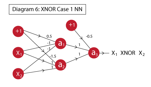
As a reminder, the truth table of XNOR function is:
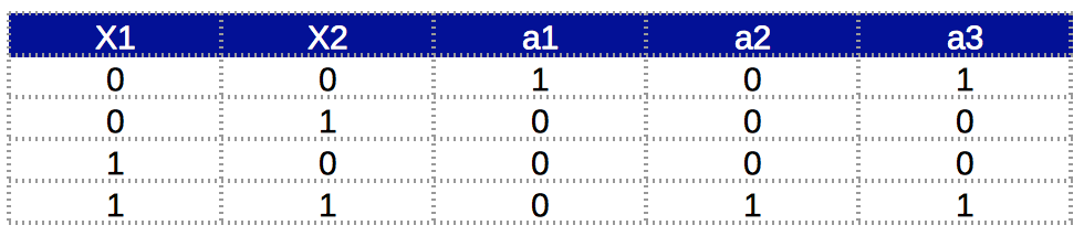
Now we will directly implement both feed forward and backward at one go.
Step 1: Define variables
import theano
import theano.tensor as T
from theano.ifelse import ifelse
import numpy as np
from random import random

#Define variables:
x = T.matrix('x')
w1 = theano.shared(np.array([random(),random()]))
w2 = theano.shared(np.array([random(),random()]))
w3 = theano.shared(np.array([random(),random()]))
b1 = theano.shared(1.)
b2 = theano.shared(1.)
learning_rate = 0.01
In this step we have defined all the required variables as in the previous case. Note that now we have 3 weight vectors corresponding to each neuron and 2 bias units corresponding to 2 layers.
Step 2: Define mathematical expression
a1 = 1/(1+T.exp(-T.dot(x,w1)-b1))
a2 = 1/(1+T.exp(-T.dot(x,w2)-b1))
x2 = T.stack([a1,a2],axis=1)
a3 = 1/(1+T.exp(-T.dot(x2,w3)-b2))
Here we have simply defined mathematical expressions for each neuron in sequence. Note that here an additional step was required where x2 is determined. This is required because we want the outputs of a1 and a2 to be combined into a matrix whose dot product can be taken with the weights vector.
Lets explore this a bit further. Both a1 and a2 would return a vector with 4 units. So if we simply take an array [a1, a2] then we’ll obtain something like [ [a11,a12,a13,a14], [a21,a22,a23,a24] ]. However, we want this to be [ [a11,a21], [a12,a22], [a13,a23], [a14,a24] ]. The stacking function of Theano does this job for us.
Step 3: Define gradient and update rule
a_hat = T.vector('a_hat') #Actual output
cost = -(a_hat*T.log(a3) + (1-a_hat)*T.log(1-a3)).sum()
dw1,dw2,dw3,db1,db2 = T.grad(cost,[w1,w2,w3,b1,b2])

train = function(
    inputs = [x,a_hat],
    outputs = [a3,cost],
    updates = [
        [w1, w1-learning_rate*dw1],
        [w2, w2-learning_rate*dw2],
        [w3, w3-learning_rate*dw3],
        [b1, b1-learning_rate*db1],
        [b2, b2-learning_rate*db2]
    ]
)
This is very similar to the previous case. The key difference being that now we have to determine the gradients of 3 weight vectors and 2 bias units and update them accordingly.
Step 4: Train the model
inputs = [
    [0, 0],
    [0, 1],
    [1, 0],
    [1, 1]
]
outputs = [1,0,0,1]

#Iterate through all inputs and find outputs:
cost = []
for iteration in range(30000):
    pred, cost_iter = train(inputs, outputs)
    cost.append(cost_iter)

#Print the outputs:
print 'The outputs of the NN are:'
for i in range(len(inputs)):
    print 'The output for x1=%d | x2=%d is %.2f' % (inputs[i][0],inputs[i][1],pred[i])

#Plot the flow of cost:
print '\nThe flow of cost during model run is as following:'
import matplotlib.pyplot as plt
%matplotlib inline
plt.plot(cost)
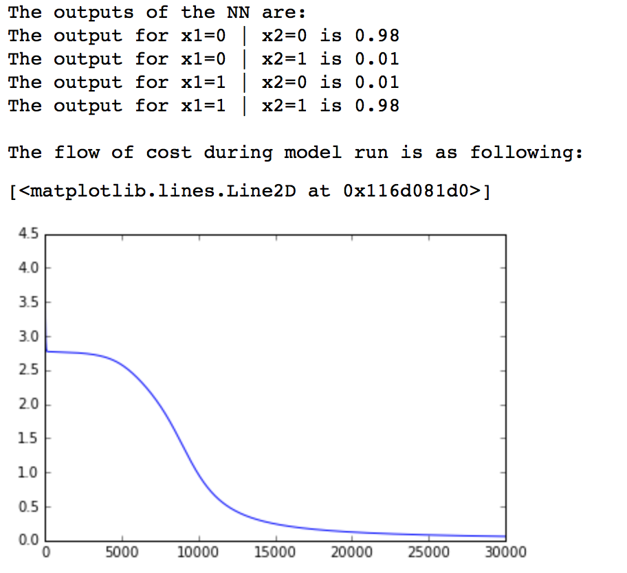
We can see that our network has successfully learned the XNOR function. Also, the cost of the model has reduced to reasonable limit. With this, we have successfully implemented a 2-layer network.
End Notes
In this article, we understood the basics of Theano package in Python and how it acts as a programming language. We also implemented some basic neural networks using Theano. I am sure that implementing Neural Networks on Theano will enhance your understanding of NN on the whole.
If hope you have been able to follow till this point, you really deserve a pat on your back. I can understand that Theano is not a traditional plug and play system like most of sklearn’s ML models. But the beauty of neural networks lies in their flexibility and an approach like this will allow you a high degree of customization in models. Some high-level wrappers of Theano do exist like Keras and Lasagne which you can check out. But I believe knowing the core of Theano will help you in using them.
Did you find this article useful ? Please feel free to share your feedback and questions below. Eagerly waiting to interact with you!
Check out Live Competitions and compete with best Data Scientists around the world.
backward propagationdeep learningforward propogationgradient descentmachine learningmatrix factorizationNeural networktheano
Aarshay Jain
05 Jul, 2020
Aarshay graduated from MS in Data Science at Columbia University in 2017 and is currently an ML Engineer at Spotify New York. He works at an intersection or applied research and engineering while designing ML solutions to move product metrics in the required direction. He specializes in designing ML system architecture, developing offline models and deploying them in production for both batch and real time prediction use cases.


Thanks Aarshay really usefull. There's a big big step from sklearn fit models and build a theano functioning model that can make confusion.. In beetwen there's keras, that permit to easily build neural network models, so maybe it could be a first step from sklearn to theano. Do you have plans for keras full tutorial ? I this case can I suggest to develop well the modelling part, from the neural network graph to the keras code with a lot of examples ? However, good job Aarshay.
Hi Gianni, Yes you are right. Keras and Lasagne are somewhere in between. I don't have immediate plans of doing Keras but if you are interested, you can do a guest blog on Keras. Lets discuss this further offline. Please drop me a note on [email protected]. Regards, Aarshay
Hi Thank you very much for this great tutorial. I just have one question. you are using the object a_hat as the actual outputs, but i cant seem to understand where the outputs are initialized in this vector? I'm probably missing something here. Can you please explain where they are been initialized?
Hi, Theano works a bit differently. Theano variables are just objects which don't hold a permanent memory. You can understand them as functions. So they get a value only when the function is called. Thus Variables are not initialized here. Whenever we call the Theano function, we pass arguments which go into the variables being used in the function. Hope this makes sense.
keep sharing such ideas in the future as well.this was actually what i was looking for,and i am glad to came here you keep up the fantastic work!my weblog..
thank you keerthi.. i'll try my best :)
Thanks for a wonderful post. My question is - For the neural network with one layer, you added the bias term in the mathematical expression i.e. z = T.dot(x,w) + b. But for the multiple layer case you subtracted the bias term i.e. a1 = 1/(1+T.exp(-T.dot(x,w1)-b1)) a2 = 1/(1+T.exp(-T.dot(x,w2)-b1)) a3 = 1/(1+T.exp(-T.dot(x2,w3)-b2)) I don't understand why it is different in both cases. Please can you explain? Thanks
You are welcome. Regarding the mathematical expression, if you observe carefully, both the T.dot(x,w1) and b1 are negative. This is because the sigmoid function is 1/(1+e(-x). There x is "T.dot(x,w1) + b1". Hope this makes sense.
Superb article...
Glad you liked it :)
can you please explain about "pred" in the AND network theano