This Machine Learning Project on Imbalanced Data Can Add Value to Your Resume

Introduction

It takes sheer courage and hard work to become a successful self-taught data scientist or to make a mid career transition. But, with growing community support, more and more people are now encouraged to make these bold career move. Do you dream to build a career in data science? Trust me, you are not alone!

Like it or not, a bitter truth about data science industry is that self-learning / certification / coursework is not sufficient to get you a job. People with little or no experience in real data science projects usually get filtered out in early stages by recruiters. This leaves self taught learners or people transitioning in a difficult place – “You need some experience on your CV to get your first data science job!” – How do you solve for it?

If you are facing this challenge, don’t let it stop you. Don’t lose hope. Here is the way out – there are several open data set repositories. With them to our disposal, we can use them tactically to build projects and make our resumes worthier. After all, recruiters are looking for proof of your knowledge.

In this article, I’ll get you started with this process. I’ll tell you how to use open data sets to create meaningful projects and improve your knowledge in this process. I’ve created this ML project (in R), which you can showcase on your resume. But, make sure that you work & develop the project from where I leave. Having a resume which stands out by doing such projects, will increase your chances of getting hired magnificently.

Note: This ML project will be most helpful to people (using R) who are actively looking for their first or next job in data science. You must have knowledge of ML algorithms. If you are already an experienced (>3 years) data scientist, you might have already worked on this / similar projects.

 

How will this project add value to your resume?

The data used in this project is imbalanced. In real life, some extremely critical situations result in imbalanced data sets. For example – fraud detection, cancer detection, manufacturing defects, online ads conversion etc. Thus, having prior experience of working on such data might rule the situation in your favor (worth a try!).

Furthermore, some characteristics of this project which makes it a worthy project include:

1. Working on imbalanced data sets is tricky. Simple classification algorithms tend to struggle in such situations.
2. The data is fairly large and high dimensional. Hence, this would help you understand & overcome machine’s memory issues.
3. This project will demonstrate your programming, data analysis and machine learning skills.
4. Working on such projects driven by self – desire will help recruiters understand:
   • You are a self motivated person
   • Mostly, self learners tend to give up. But, you have really put in hard work to reach where you are.

If not job, this project will give you enough confidence & knowledge that you can build more ML projects on your own. Once you have completed this project, put in on your GitHub repo and showcase it to the world. Leave the link in the comments below to showcase your motivation – you never know when a recruiter drops by!

Note: If you are new to imbalanced classification problems. I recommend you to read this article.

 

Table of Contents

1. Problem Statement & Hypothesis Generation
2. Data Exploration
3. Data Cleaning
   • Missing Value Imputation
4. Data Manipulation a.k.a Feature Engineering
5. Machine Learning
   • Imbalanced Techniques
     • Oversampling
     • Undersampling
     • SMOTE
   • naive Bayes
   • XgBoost
     • Homework – Top 20 Features
     • AUC Threshold
   • SVM
     • Homework – Class weights

 

1. Problem Statement and Hypothesis Generation

The Problem Statement

Given various features, the aim is to build a predictive model to determine the income level for people in US. The income levels are binned at below 50K and above 50K.

From the problem statement, it’s evident that this is a binary classification problem.

Generating hypothesis is the most crucial step in building models. Yet, most analysts tend to overlook this step. In simple words, this technique enlightens our way by indicating which direction (set of variables) to choose.

This step should be practiced before looking at the data. This is done to think broadly and not be constrained by what is available. In this step, we’ll create a laundry list of factors which we think could influence the prediction metrics. Read more about hypothesis generation here.

Let’s think of some hypothesis which can influence the outcome. Here is a set of hypothesis to get you started:

Hò : There is no significant impact of the variables (below) on the dependent variable.

Ha : There exists a significant impact of the variables (below) on the dependent variable.

1. Age
2. Marital Status
3. Income
4. Family Members
5. No. of Dependents
6. Tax Paid
7. Investment (Mutual Fund, Stock)
8. Return from Investments
9. Education
10. Spouse Education
11. Nationality
12. Occupation
13. Region in US
14. Race
15. Occupation category

Remind you, this is not an exhaustive list. I’d suggest you not to limit your thoughts with the ones above, your aim should be to make your project as comprehensive & presentable as possible.

Also, every time you think of an hypothesis, try and think of what would be the relationship like and why would that hypothesis stand true. For example, when I say Education – what I really mean is this: “I think that with higher education, people would have higher chances of better employment and hence their income would have higher chances of being more than 50K.”

Similarly, spend some time thinking about your set of hypothesis, how would they be impacting income and hence what is the best way to capture the mathematical relationship.

P.S. Do this before you move forward in the article

 

2. Data Exploration

For this project, we’ve taken the data set from UCI Machine Learning Repository: Data set information. The first step is to look at the data and identify which of our hypothesis are available in the data.

If you’ve used this data repository in past, you would know that downloading and modeling data isn’t as easy as it might look. If you download the data from link given above, you’d find that column headers are missing. Therefore, for your convenience, I’ve provided the link for workable version of test and train data:

Download Train Data
Download Test Data

As mentioned above, we’ll use R for this project. Now, we’ll load the data into R and look at it closely.

#set working directory
> path <- "C:/Users/manish/Desktop/Data/MLP"
> setwd(path)

#load packages & data
> library(data.table)
> train <- fread("train.csv",na.strings = c(""," ","?","NA",NA))
> test <- fread("test.csv",na.strings = c(""," ","?","NA",NA))

#look at data
> dim(train); str (train); View(train)
> dim(test); str (test); View(test)

We see that train data has 199523 rows & 41 columns. Test data has 99762 rows and 41 columns. Generally, test data comes with one less column than train. It means that this data set has test prediction values also. This will help us in evaluating our model.

#check first few rows of train & test
> train[1:5]
> test [1:5]

#check target variables
> unique(train$income_level)
[1] "-50000" "+50000"
> unique(test$income_level)
[1] "-50000"  "50000+."

The denominations of these target levels aren’t same. This disparity will cause trouble in model evaluation. Being a binary classification problem, we can encode these variables as 0 and 1.

#encode target variables
> train[,income_level := ifelse(income_level == "-50000",0,1)]
> test[,income_level := ifelse(income_level == "-50000",0,1)]

Let’s look at the severity of imbalanced classes in our data:

> round(prop.table(table(train$income_level))*100)
   0      1
   94     6

We see that the majority class has a proportion of 94%. In other words, with a decent ML algorithm, our model would get 94% model accuracy. In absolute figures, it looks incredible. But, our performance would depend on, how good can we predict the minority classes. More on this in coming sections!

As seen in str() above, the columns in the both data set aren’t as per column classes given on data set page. Let’s update the column classes accordingly. data.table package offers fast and simple way to make changes in multiple columns at once.

#set column classes
> factcols <- c(2:5,7,8:16,20:29,31:38,40,41)
> numcols <- setdiff(1:40,factcols)

> train[,(factcols) := lapply(.SD, factor), .SDcols = factcols]
> train[,(numcols) := lapply(.SD, as.numeric), .SDcols = numcols]

> test[,(factcols) := lapply(.SD, factor), .SDcols = factcols]
> test[,(numcols) := lapply(.SD, as.numeric), .SDcols = numcols]

Now, let’s separate categorical variables & numerical variables. This will help us in further analysis.

#subset categorical variables
> cat_train <- train[,factcols, with=FALSE]
> cat_test <- test[,factcols,with=FALSE]

#subset numerical variables
> num_train <- train[,numcols,with=FALSE]
> num_test <- test[,numcols,with=FALSE] > rm(train,test) #to save memory

Removing train and test files would allow us to use our memory for other computational purposes which was earlier held up by these data sets.

Let’s begin with numerical data now. The best way to understand these variables is using Histogram.

#load libraries
> library(ggplot2)
> library(plotly)

#write a plot function
> tr <- function(a){
            ggplot(data = num_train, aes(x= a, y=..density..)) + geom_histogram(fill="blue",color="red",alpha = 0.5,bins =100) + geom_density()
 ggplotly()
}

For ease of understanding, we’ve created a histogram overlapped with density curve. This curve will helps us decipher the distribution pattern more clearly. ggplotly() package will make our resultant plots interactive, thereby saving us lot of time. Let’s look at some variables:

#variable age
> tr(num_train$age)

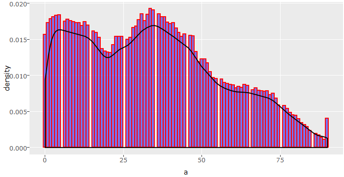
As we can see, the data set consists of people aged from 0 to 90 with frequency of people declining with age. Now, if we think of the problem we are trying to solve, do you think population below age 20 could earn >50K under normal circumstances? I don’t think so. Therefore, we can bin this variable into age groups.

#variable capital_losses
> tr(num_train$capital_losses)

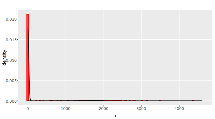
This is a nasty right skewed graph. In skewed distribution, normalizing is always an option. But, we need to look into this variable deeper as this insight isn’t significant enough for decision making. One option could be, to check for unique values. If they are less, we can tabulate the distribution (done in upcoming sections).

Furthermore, in classification problems, we should also plot numerical variables with dependent variable. This would help us determine the clusters (if exists) of classes 0 and 1. For this, we need to add the target variable in num_train data:

#add target variable
> num_train[,income_level := cat_train$income_level]

#create a scatter plot
> ggplot(data=num_train,aes(x = age, y=wage_per_hour))+geom_point(aes(colour=income_level))+scale_y_continuous("wage per hour", breaks = seq(0,10000,1000))

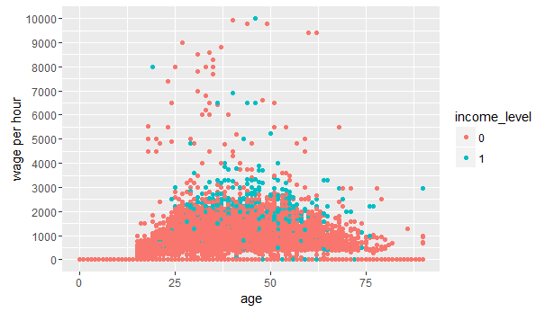
As we can see, most of the people having income_level 1, seem to fall in the age of 25-65 earning wage of $1000 to $4000 per hour. This plot further strengthens our assumption that age < 20 would have income_level 0, hence we will bin this variable.

Identifying hidden trends is easier said than done. We need to look at a variable(s) from different angles to spot the hidden trends. Don’t stop here. I suggest you to plot all variables and understand their distribution. This would give us enough idea for doing feature engineering.

Similarly, we can visualize our categorical variables as well. For categories, rather than a bland bar chart, a dodged bar chart provides more information. In dodged bar chart, we plot the categorical variables & dependent variable adjacent to each other.

#dodged bar chart
> all_bar <- function(i){
 ggplot(cat_train,aes(x=i,fill=income_level))+geom_bar(position = "dodge",  color="black")+scale_fill_brewer(palette = "Pastel1")+theme(axis.text.x =element_text(angle  = 60,hjust = 1,size=10))
}

#variable class_of_worker
> all_bar(cat_train$class_of_worker)

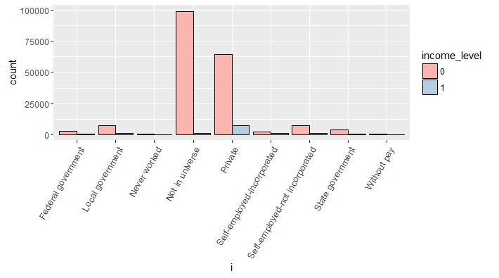
Though, no specific information is provided about Not in universe category. Let’s assume that, this response is given by people who got frustrated (due to any reason) while filling their census data. This variable looks imbalanced i.e. only two category levels seem to dominate. In such situation, a good practice is to combine levels having less than 5% frequency of the total category frequency.

#variable education
> all_bar(cat_train$education)

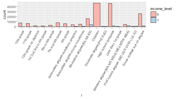
Evidently, all children have income_level 0. Also, we can infer than Bachelors degree holders have the largest proportion of people have income_level 1. Similarly, you can plot other categorical variables also.

Alternative way of checking categories is using 2 way tables. Yes, you can create proportionate tables to check the effect of dependent variable per categories as shown:

> prop.table(table(cat_train$marital_status,cat_train$income_level),1)
> prop.table(table(cat_train$class_of_worker,cat_train$income_level),1)

 

3. Data Cleaning

Let’s check for missing values in numeric variables.

#check missing values in numerical data
> table(is.na(num_train))
> table(is.na(num_test))

We see that numeric variables has no missing values. Good for us! While working on numeric variables, a good practice is to check for correlation in numeric variables. caret package offers a convenient way to filter out variables with high correlation. Let’s see:

> library(caret)

#set threshold as 0.7
> ax <-findCorrelation(x = cor(num_train), cutoff = 0.7)

> num_train <- num_train[,-ax,with=FALSE] 
> num_test[,weeks_worked_in_year := NULL]

The variable weeks_worked_in_year gets removed. For hygiene purpose, we’ve removed that variable from test data too. It’s not necessary though!

Now, let’s check for missing values in categorical data. We’ll use base sapply() to find out percentage of missing values per column.

#check missing values per columns
> mvtr <- sapply(cat_train, function(x){sum(is.na(x))/length(x)})*100
> mvte <- sapply(cat_test, function(x){sum(is.na(x)/length(x))}*100)
> mvtr
> mvte

We find that some of the variables have ~50% missing values. High proportion of missing value can be attributed to difficulty in data collection. For now, we’ll remove these category levels. A simple subset() function does the trick.

#select columns with missing value less than 5%
> cat_train <- subset(cat_train, select = mvtr < 5 )
> cat_test <- subset(cat_test, select = mvte < 5)

For the rest of missing values, a nicer approach would be to label them as ‘Unavailable’. Imputing missing values on large data sets can be painstaking. data.table’s set() function makes this computation insanely fast.

#set NA as Unavailable - train data
#convert to characters
> cat_train <- cat_train[,names(cat_train) := lapply(.SD, as.character),.SDcols = names(cat_train)]
> for (i in seq_along(cat_train)) set(cat_train, i=which(is.na(cat_train[[i]])), j=i, value="Unavailable")
#convert back to factors
> cat_train <- cat_train[, names(cat_train) := lapply(.SD,factor), .SDcols = names(cat_train)]

#set NA as Unavailable - test data
> cat_test <- cat_test[, (names(cat_test)) := lapply(.SD, as.character), .SDcols = names(cat_test)]
> for (i in seq_along(cat_test)) set(cat_test, i=which(is.na(cat_test[[i]])), j=i, value="Unavailable")
#convert back to factors
> cat_test <- cat_test[, (names(cat_test)) := lapply(.SD, factor), .SDcols = names(cat_test)]

 

4. Data Manipulation

We are approaching towards machine learning stage. But, machine learning algorithms return better accuracy when the data set has clear signals to offer. Specially, in case of imbalanced classification, we should try our best to shape the data such that we can derive maximum information about minority class.

In previous analysis, we saw that categorical variables have several levels with low frequencies. Such levels don’t help as chances are they wouldn’t be available in test set. We’ll do this hygiene check anyways, in coming steps. To combine levels, a simple for loop does the trick. After combining, the new category level will named as ‘Other’.

#combine factor levels with less than 5% values
#train
> for(i in names(cat_train)){
                  p <- 5/100
                  ld <- names(which(prop.table(table(cat_train[[i]])) < p))
                  levels(cat_train[[i]])[levels(cat_train[[i]]) %in% ld] <- "Other"
}

#test
> for(i in names(cat_test)){
                  p <- 5/100
                  ld <- names(which(prop.table(table(cat_test[[i]])) < p))
                  levels(cat_test[[i]])[levels(cat_test[[i]]) %in% ld] <- "Other"
}

Time for hygiene check. Let’s check if there exists a mismatch between categorical levels in train and test data. Either you can write a function for accomplish this. We’ll rather use a hack derived from mlr package.

#check columns with unequal levels
library(mlr)
> summarizeColumns(cat_train)[,"nlevs"]
> summarizeColumns(cat_test)[,"nlevs"]

The parameter “nlevs” returns the unique number of level from the given set of variables.

Before proceeding to the modeling stage, let’s look at numeric variables and reflect on possible ways for binning. Since a histogram wasn’t enough for us to make decision, let’s create simple tables representing counts of unique values in these variables as shown:

> num_train[,.N,age][order(age)]
> num_train[,.N,wage_per_hour][order(-N)]

Similarly, you should check other variables also. After this activity, we are clear that more than 70-80% of the observations are 0 in these variables. Let’s bin these variables accordingly. I used a decision tree to determine the range of resultant bins. However, it will be interested to see how 0-25, 26-65, 66-90 works (discerned from plots above).  You should try it sometime later!

#bin age variable 0-30 31-60 61 - 90
> num_train[,age:= cut(x = age,breaks = c(0,30,60,90),include.lowest = TRUE,labels = c("young","adult","old"))]
> num_train[,age := factor(age)]

> num_test[,age:= cut(x = age,breaks = c(0,30,60,90),include.lowest = TRUE,labels = c("young","adult","old"))]
> num_test[,age := factor(age)]

#Bin numeric variables with Zero and MoreThanZero
> num_train[,wage_per_hour := ifelse(wage_per_hour == 0,"Zero","MoreThanZero")][,wage_per_hour := as.factor(wage_per_hour)]
> num_train[,capital_gains := ifelse(capital_gains == 0,"Zero","MoreThanZero")][,capital_gains := as.factor(capital_gains)]
> num_train[,capital_losses := ifelse(capital_losses == 0,"Zero","MoreThanZero")][,capital_losses := as.factor(capital_losses)]
> num_train[,dividend_from_Stocks := ifelse(dividend_from_Stocks == 0,"Zero","MoreThanZero")][,dividend_from_Stocks := as.factor(dividend_from_Stocks)]

> num_test[,wage_per_hour := ifelse(wage_per_hour == 0,"Zero","MoreThanZero")][,wage_per_hour := as.factor(wage_per_hour)]
> num_test[,capital_gains := ifelse(capital_gains == 0,"Zero","MoreThanZero")][,capital_gains := as.factor(capital_gains)]
> num_test[,capital_losses := ifelse(capital_losses == 0,"Zero","MoreThanZero")][,capital_losses := as.factor(capital_losses)]
> num_test[,dividend_from_Stocks := ifelse(dividend_from_Stocks == 0,"Zero","MoreThanZero")][,dividend_from_Stocks := as.factor(dividend_from_Stocks)]

Now, we can remove the dependent variable from num_train, we added for visualization purpose earlier.

> num_train[,income_level := NULL]

 

5. Machine Learning

Making predictions on this data should atleast give us ~94% accuracy. However, while working on imbalanced problems, accuracy is considered to be a poor evaluation metrics because:

1. Accuracy is calculated by ratio of correct classifications / incorrect classifications.
2. This metric would largely tell us how accurate our predictions are on the majority class (since it comprises 94% of values). But, we need to know if we are predicting minority class correctly. We’re doomed here.

In such situations, we should use elements of confusion matrix.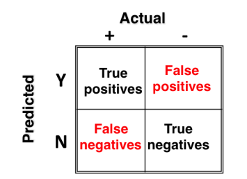 

Following are the metrics we’ll use to evaluate our predictive accuracy:

• Sensitivity = True Positive Rate (TP/TP+FN) – It says, ‘out of all the positive (majority class) values, how many have been predicted correctly’.
• Specificity = True Negative Rate (TN/TN +FP) – It says, ‘out of all the negative (minority class) values, how many have been predicted correctly’.
• Precision = (TP/TP+FP)
• Recall = Sensitivity
• F score = 2 * (Precision * Recall)/ (Precision + Recall) – It is the harmonic mean of precision and recall. It is used to compare several models side-by-side. Higher the better.

In quest of better accuracy, we’ll use various techniques used on imbalanced classification. For modeling purpose, we’ll use the fantastic mlr package, which I use(over) these days. I hope you’ve read the recommended article mentioned above because if you are unfamiliar with these techniques, chances are you would lose the way moving forward.

#combine data and make test & train files
> d_train <- cbind(num_train,cat_train)
> d_test <- cbind(num_test,cat_test)

#remove unwanted files
> rm(num_train,num_test,cat_train,cat_test) #save memory

#load library for machine learning
> library(mlr)

#create task
> train.task <- makeClassifTask(data = d_train,target = "income_level")
> test.task <- makeClassifTask(data=d_test,target = "income_level")

#remove zero variance features
> train.task <- removeConstantFeatures(train.task)
> test.task <- removeConstantFeatures(test.task)

#get variable importance chart
> var_imp <- generateFilterValuesData(train.task, method = c("information.gain"))
> plotFilterValues(var_imp,feat.type.cols = TRUE)

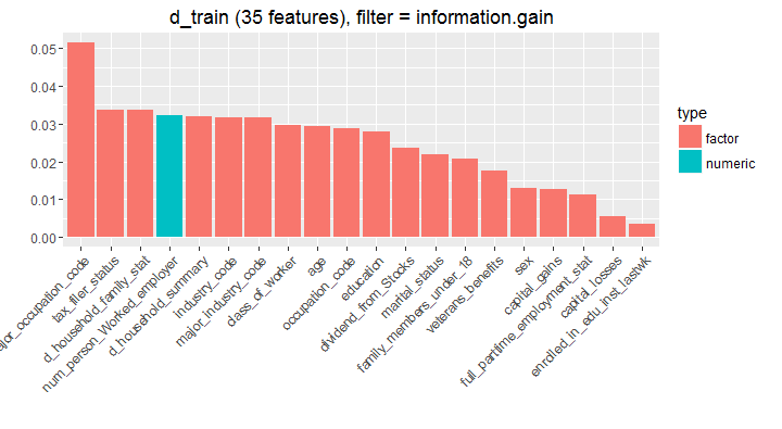
In simple words, you can understand that the variable major_occupation_code would provide highest information to the model followed by other variables in descending order. This chart is deduced using a tree algorithm, where at every split, the information is calculated using reduction in entropy (homogeneity). Let’s keep this knowledge safe, we might use it in coming steps.

Now, we’ll try to make our data balanced using various techniques such as over sampling, undersampling and SMOTE. In SMOTE, the algorithm looks at n nearest neighbors, measures the distance between them and introduces a new observation at the center of n observations. While proceeding, we must keep in mind that these techniques have their own drawbacks such as:

• undersampling leads to loss of information
• oversampling leads to overestimation of minority class

Being your first project(hopefully), we should try all techniques and experience how it affects.

#undersampling 
> train.under <- undersample(train.task,rate = 0.1) #keep only 10% of majority class
> table(getTaskTargets(train.under))

#oversampling
> train.over <- oversample(train.task,rate=15) #make minority class 15 times
> table(getTaskTargets(train.over))

#SMOTE
> train.smote <- smote(train.task,rate = 15,nn = 5)

Looks like, my machine gave up at these SMOTE parameters. It’s been over 50 minutes and this code hasn’t executed. Look at the havoc this is creating in my poor machine:

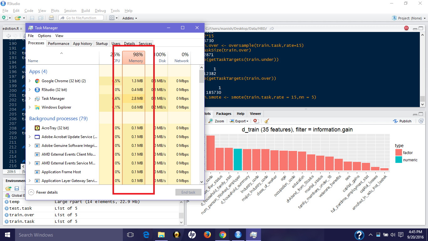
While working on such data sets, it’s important for you to learn the ways to hop such obstacles. Let’s modify the parameters and run it again:

> system.time(
    train.smote <- smote(train.task,rate = 10,nn = 3) 
   )
Warning messages:
# 1: In is.factor(x) :
# Reached total allocation of 8084Mb: see help(memory.size)
# 2: In is.factor(x) :
# Reached total allocation of 8084Mb: see help(memory.size)
# user system elapsed
# 81.95 21.86 184.56
> table(getTaskTargets(train.smote))

It did run with some warning messages. We can ignore them for now.  Let’s now look at the available algorithms we can use to solve this problem.

#lets see which algorithms are available
> listLearners("classif","twoclass")[c("class","package")]

We’ll start with naive Bayes, an algorithms based on bayes theorem. In case of high dimensional data like text-mining, naive Bayes tends to do wonders in accuracy. It works on categorical data. In case of numeric variables, a normal distribution is considered for these variables and a mean and standard deviation is calculated. Then, using some standard z-table calculations probabilities can be estimated for each of your continuous variables to make the naive Bayes classifier.

We’ll use naive Bayes on all 4 data sets (imbalanced, oversample, undersample and SMOTE) and compare the prediction accuracy using cross validation.

#naive Bayes
> naive_learner <- makeLearner("classif.naiveBayes",predict.type = "response")
> naive_learner$par.vals <- list(laplace = 1)

#10fold CV - stratified
> folds <- makeResampleDesc("CV",iters=10,stratify = TRUE)

#cross validation function
> fun_cv <- function(a){
     crv_val <- resample(naive_learner,a,folds,measures = list(acc,tpr,tnr,fpr,fp,fn))
     crv_val$aggr
}

> fun_cv (train.task)
# acc.test.mean tpr.test.mean tnr.test.mean fpr.test.mean
# 0.7337249       0.8954134     0.7230270    0.2769730

> fun_cv(train.under)
# acc.test.mean tpr.test.mean tnr.test.mean fpr.test.mean
# 0.7637315      0.9126978     0.6651696     0.3348304

> fun_cv(train.over)
# acc.test.mean tpr.test.mean tnr.test.mean fpr.test.mean
#   0.7861459     0.9145749     0.6586852    0.3413148

> fun_cv(train.smote)
# acc.test.mean tpr.test.mean tnr.test.mean fpr.test.mean
#   0.8562135     0.9168955    0.8160638     0.1839362

This package names cross validated results are test.mean. After comparing, we see that train.smote gives the highest true positive rate and true negative rate. Hence, we learn that SMOTE technique outperforms the other two sampling methods.

Now, let’s build our model SMOTE data and check our final prediction accuracy.

#train and predict
> nB_model <- train(naive_learner, train.smote)
> nB_predict <- predict(nB_model,test.task)

#evaluate
> nB_prediction <- nB_predict$data$response
> dCM <- confusionMatrix(d_test$income_level,nB_prediction)
# Accuracy : 0.8174
# Sensitivity : 0.9862
# Specificity : 0.2299

#calculate F measure
> precision <- dCM$byClass['Pos Pred Value']
> recall <- dCM$byClass['Sensitivity']

> f_measure <- 2*((precision*recall)/(precision+recall))
> f_measure 

The function confusionMatrix is taken from library(caret). This naive Bayes model predicts 98% of the majority class correctly, but disappoints at minority class prediction (~23%). Let us not get hopeless and try more techniques to improve our accuracy. Remember, the more you hustle, better you get!

Let’s use xgboost algorithm and try to improve our model. We’ll do 5 fold cross validation and 5 round random search for parameter tuning. Finally, we’ll build the model using the best tuned parameters.

#xgboost
> set.seed(2002)
> xgb_learner <- makeLearner("classif.xgboost",predict.type = "response")
> xgb_learner$par.vals <- list(
                      objective = "binary:logistic",
                      eval_metric = "error",
                      nrounds = 150,
                      print.every.n = 50
)

#define hyperparameters for tuning
> xg_ps <- makeParamSet( 
                makeIntegerParam("max_depth",lower=3,upper=10),
                makeNumericParam("lambda",lower=0.05,upper=0.5),
                makeNumericParam("eta", lower = 0.01, upper = 0.5),
                makeNumericParam("subsample", lower = 0.50, upper = 1),
                makeNumericParam("min_child_weight",lower=2,upper=10),
                makeNumericParam("colsample_bytree",lower = 0.50,upper = 0.80)
)

#define search function
> rancontrol <- makeTuneControlRandom(maxit = 5L) #do 5 iterations

#5 fold cross validation
> set_cv <- makeResampleDesc("CV",iters = 5L,stratify = TRUE)

#tune parameters
> xgb_tune <- tuneParams(learner = xgb_learner, task = train.task, resampling = set_cv, measures = list(acc,tpr,tnr,fpr,fp,fn), par.set = xg_ps, control = rancontrol)
# Tune result:
# Op. pars: max_depth=3; lambda=0.221; eta=0.161; subsample=0.698; min_child_weight=7.67; colsample_bytree=0.642
# acc.test.mean=0.948,tpr.test.mean=0.989,tnr.test.mean=0.324,fpr.test.mean=0.676

Now, we can use these parameter for modeling using xgb_tune$x which contains the best tuned parameters.

#set optimal parameters
> xgb_new <- setHyperPars(learner = xgb_learner, par.vals = xgb_tune$x)

#train model
> xgmodel <- train(xgb_new, train.task)

#test model
> predict.xg <- predict(xgmodel, test.task)

#make prediction
> xg_prediction <- predict.xg$data$response

#make confusion matrix
> xg_confused <- confusionMatrix(d_test$income_level,xg_prediction)
Accuracy : 0.948
Sensitivity : 0.9574
Specificity : 0.6585


> precision <- xg_confused$byClass['Pos Pred Value']
> recall <- xg_confused$byClass['Sensitivity']

> f_measure <- 2*((precision*recall)/(precision+recall))
> f_measure
#0.9726374 

As we can see, xgboost has outperformed naive Bayes model’s accuracy (as expected!). Can we further improve ?

Until now, we’ve used all the variables in the data. Shall we try using the important ones? Consider it your homework. Let me provide you hint to do this:

#top 20 features
> filtered.data <- filterFeatures(train.task,method = "information.gain",abs = 20)
#train
> xgb_boost <- train(xgb_new,filtered.data)

After this, follow the same steps as above for predictions and evaluation. Tell me your understanding in comments below.

Until now, our model has been making label predictions. The threshold used for making these predictions in 0.5 as seen by:

> predict.xg$threshold
[[1]] 0.5

Due to imbalanced nature of the data, the threshold of 0.5 will always favor the majority class since the probability of a class 1 is quite low. Now, we’ll try a new technique:

• Instead of labels, we’ll predict probabilities
• Plot and study the AUC curve
• Adjust the threshold for better prediction

We’ll continue using xgboost for this stunt. To do this, we need to change the predict.type parameter while defining learner.

#xgboost AUC
> xgb_prob <- setPredictType(learner = xgb_new,predict.type = "prob")

#train model
> xgmodel_prob <- train(xgb_prob,train.task)

#predict
> predict.xgprob <- predict(xgmodel_prob,test.task)

Now, let’s look at the probability table thus created:

#predicted probabilities
> predict.xgprob$data[1:10,]

Since, we have obtained the class probabilities, let’s create an AUC curve and determine the basis to modify prediction threshold.

> df <- generateThreshVsPerfData(predict.xgprob,measures = list(fpr,tpr))
> plotROCCurves(df)

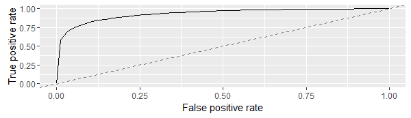
AUC is a measure of true positive rate and false positive rate. We aim to reach as close to top left corner as possible. Therefore, we should aim to reduce the threshold so that the false positive rate can be reduced.

#set threshold as 0.4
> pred2 <- setThreshold(predict.xgprob,0.4)
> confusionMatrix(d_test$income_level,pred2$data$response)
# Sensitivity : 0.9512
# Specificity : 0.7228

With 0.4 threshold, our model returned better predictions than our previous xgboost model at 0.5 threshold. Thus, you can see that setting threshold using AUC curve actually affect our model performance. Let’s give one more try.

> pred3 <- setThreshold(predict.xgprob,0.30)
> confusionMatrix(d_test$income_level,pred3$data$response)
#Accuracy : 0.944
# Sensitivity : 0.9458
# Specificity : 0.7771

This model has outperformed all our models i.e. in other words, this is the best model because 77% of the minority classes have been predicted correctly.

Similarly, you can try and test other threshold values to check if your model improves. In this xgboost model, there is a lot you can do such as:

• Increase the number of rounds
• Do 10 fold CV
• Increase repetitions in random search
• Build models on other 3 data sets and see which one is better

Apart from the methods listed above, you can also assign class weights such that the algorithm pays more attention while classifying the class with higher weight. I leave this part as homework to you. Run the code below and update me if you model surpassed our previous xgboost prediction. Use SVM in homework. An important tip: The code below might take longer than expected to run, therefore close all other applications.

#use SVM
> getParamSet("classif.svm")
> svm_learner <- makeLearner("classif.svm",predict.type = "response")
> svm_learner$par.vals<- list(class.weights = c("0"=1,"1"=10),kernel="radial")

> svm_param <- makeParamSet(
            makeIntegerParam("cost",lower = 10^-1,upper = 10^2), 
            makeIntegerParam("gamma",lower= 0.5,upper = 2)
)

#random search
> set_search <- makeTuneControlRandom(maxit = 5L) #5 times

#cross validation #10L seem to take forever
> set_cv <- makeResampleDesc("CV",iters=5L,stratify = TRUE)

#tune Params
> svm_tune <- tuneParams(learner = svm_learner,task = train.task,measures = list(acc,tpr,tnr,fpr,fp,fn), par.set = svm_param,control = set_search,resampling = set_cv)
)

#set hyperparameters
>svm_new <- setHyperPars(learner = svm_learner, par.vals = svm_tune$x)

#train model
>svm_model <- train(svm_new,train.task)

#test model
>predict_svm <- predict(svm_model,test.task)

> confusionMatrix(d_test$income_level,predict_svm$data$response)

 

End Notes

I hope this project will helped you understand the importance of data exploration, visualization, manipulation in machine learning. To showcase this project on your resume, create your github account, upload this project along with important findings. I have not deliberately provided my code so that you write it at your end.

Make sure you understand this project and develop on it further. Recruiter can figure out who’s honest and not. And trust me, such projects will different your profile from other candidates.

If you want me to create and share more such machine learning projects, write your suggestion on problem types below. I’d love work on something which you think is challenging and would like to conquer it.

Looking for a job in analytics? Check out currently hiring jobs in machine learning and data science