Complete Study of Factors Contributing to Air Pollution

Introduction

The air pollution is one of the main causes of death in the world. Several cities are on the radar of WHO, which are about to touch the dangerous level. Sadly, India is one of the countries with maximum number of most polluted cities in the world.

Especially, on the onset of Diwali, the air quality index of  DelhiNCR soars to new heights. This year the air quality index has already crossed last year’s post Diwali index.

To know the intricacies of the problem, we decided to do an analytical study for the factors that contribute most to air pollution in New Delhi.

In this article, we share a case study on “Identifying Patterns in New Delhi’s Air Pollution”, in which we closely studied the air quality data for New Delhi, identified patterns, factors that lead to rise in air pollution across three key locations in New Delhi. The article also includes, impact of the Delhi Government’s initiative “Odd-Even Pilot Project Phase II” to tackle the problem of air pollution.

On this occasion of Diwali, we want to sensitize the readers towards celebrating environmentally safe Diwali this year.

Table of Contents

1. Overview

• Problem Statement
• Objective and Scope of the Project
• Data Sources
• Tools and Techniques
• Limitations

2. Data Description and Preparation

• Data Management
• Data Table
• Data Quality
• Data Preparations

3. Exploratory Data Analysis

• Impact of Vehicle Density & Vehicle Population
• Histogram & Box Plots
• Seasonality Analysis
• Correlation Matrix and Analysis

4. Predictive Model Development

• Multiple Linear Regression & Neural Network Models & Results
• Validation
• Conclusion
• Recommendations

5. Odd-Even Campaign

• Average Pollution Analysis
• Pollution Level Trend Analysis
• PM 2.5 & PM 10 – Before & After Campaign
• Odd-Even Impact on Traffic
• Bio-Mass Residual Burning impact on Pollution Levels
• Quantifying the Bio-Mass burning Campaign
• Sentiment Analysis on Odd-Even Campaign
• Conclusions
• Recommendations

1. Overview

The rate at which urban air pollution has grown across India is alarming. A vast majority of cities are caught in the toxic web as air quality fails to meet health-based standards. Almost all cities are reeling under severe particulate pollution while newer pollutants like oxides of nitrogen and air toxics have begun to add to the public health challenge.

According to WHO, India ranks among the world’s most polluted countries. Out of the 20 most polluted cities in the world, 13 are in India. In which, Delhi is the most polluted city in the world today.

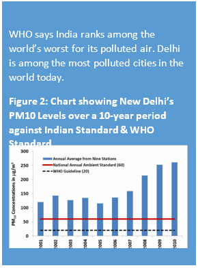
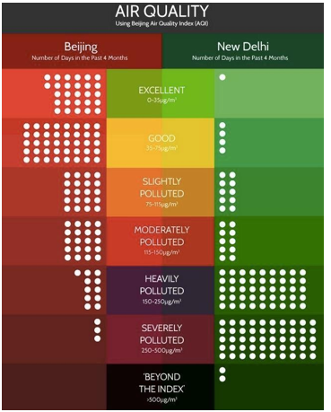
                                                 Figure: Chart showing the Air Quality Index for Beijing and New Delhi for a 4 Month period

Exposure to particulate matter for a long time can lead to respiratory and cardiovascular diseases such as asthma, bronchitis, lung cancer and heart attack. Last year, the Global Burden of Disease study pinned outdoor air pollution as the fifth largest killer in India, after high blood pressure, indoor air pollution, tobacco smoking, and poor nutrition. In 2010, about 620,000 early deaths in India occurred from air pollution-related diseases. The Central Pollution Control Board (CPCB) sponsored the study that links the pollutants, pm 10 (particulate matter smaller than 10 microns), the cause of these diseases. The central regulatory authority recently regulated stricter norms for a number of air toxins and pollutants but omitted revision of the standard for pm 10.

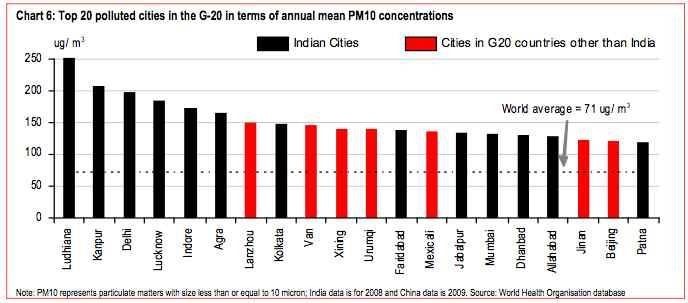Figure: Chart showing Top 20 polluted cities in the G-20 Countries in terms of annual mean PM10

Sunita Narain (Director General) Centre for Science and Environment (CSE) says, “This data confirms our worst fears about how hazardous air pollution is in our region”. In addition to this, Narain points out, 18 million years of healthy lives are lost due to illness burden that enhances the economic cost of pollution. Half of these deaths have been caused by ischemic heart disease triggered by exposure to air pollution and the rest due to stroke, chronic obstructive pulmonary disease, lower respiratory track infection and lung cancer.

• Problem Statement

We feel, if we closely study the Air Quality Data, we should be able to identify patterns (spike in air pollution levels) and identify correlating factors on key levels of Air Pollution across New Delhi. Also as part of the exercise, we wanted to study the impact of Government sponsored Initiatives like ‘Odd-Even’ Pilot Project Phase II. The Phase I of the ‘Odd- Even’ experiment was a huge success in terms of people compliance and reduction of traffic congestion, it had very little impact on the Air Pollution levels during the Campaign period.

It is also important to understand the behaviour of meteorological parameters in the planetary boundary layer because, atmosphere is the medium in which air pollutants are transported away from the source, which is governed by the meteorological parameters such as atmospheric wind speed, wind direction, and temperature.

Air pollutants are being let out into the atmosphere from a variety of sources, and the concentration of pollutants in the ambient air depends not only on the quantities that are emitted but also the ability of the atmosphere, either to absorb or disperse these pollutants.

There were conflicting reports in media on the actual cause of air pollution in New Delhi. Some sections claimed vehicles as the main source of pollution, while others held road dust & construction debris responsible. But the root cause of the problem is Industrial pollution.

Through this study, we hope to develop some insights that can help organizations (State / Central Pollution Control Boards & NGOs) to advocate more stringent policies to control air pollution.

• Objective and Scope of the Project

  1. Objective

The primary objectives of the study are:

• Study Air Pollution Data for various locations in New Delhi to identify patterns of spike in Air Pollution levels w.r.t to various monitored parameters
• Identify the Meteorological factors that correlate with the air pollution levels for the respective locations
• Explore the possibility of developing a Predictive Model for predicting the levels for key pollutants like PM 5
• Study the Odd-Even Pilot Project (Phase II) and its impact on air pollution levels in New Delhi. As part of this, also study the people’s response to this by studying the social conversation around ‘Odd-Even’

      2. Scope

• The scope of the study covers 3 major polluting centers in New Delhi
• The study covers one-year Data starting from 1st April’15. This is done to ensure seasonality factors are covered
• The Study’s focus is on factors for which authentic secondary data are available that can be used for Statistical Analysis

     3. Out of Scope:

• Experimental measures like developing first-hand data are not considered i.e. factors like Vehicle density during the given period at each location, measuring & monitoring level of road dust, Industrial pollution
• The scope of the study will cover 3 to 4 major cities in India and will include 2-3 key monitoring stations per city (depending on the data availability)
• The study will cover up to one year data starting 1st April’15 to 31st March’16. This is done to ensure seasonality factors are covered

• Data Source

The data for the Project was obtained from the website of Central Pollution Control Board (CPCB). Currently, CPCB tracks the Air Pollution levels across 23 dimension (variables). Day wise, hour wise (for some variables). Data is available on-line across the following dimensions:

1. Nitric Oxide (NO)
2. Carbon Monoxide(CO)
3. Suspended Particulate Matter/RPM/PM10
4. Nitrogen Dioxide (No2)
5. Ozone
6. Sulphur Dioxide (SO2)
7. PM 2.5 (DUST 5)
8. Toluene
9. Ethyl Benzene (Ethylben)
10. M & P Xylene
11. Oxylene
12. Oxides of Nitrogen (Nox)
13. PM10 DUST
14. PM10 RSPM
15. Ammonia NM3
16. Non Methane Hydro Carbon (NMHC)
17. Total Hydro carbon (THC)
18. Relative Humidity (RH)
19. Temperature
20. Wind Speed (Wind speed S)
21. Vertical Wind speed (Wind speed V)
22. Wind Direction
23. Solar Radiation

Not all monitoring stations track Air Pollution on all the above mentioned parameters and for all days.

India’s Central Pollution Control Board now routinely monitors four air pollutants namely Sulphur dioxide (SO2), oxides of nitrogen (NOx), suspended particulate matter (SPM) and respirable particulate matter (PM10) & (PM 2.5). These are target air pollutants for regular monitoring at 308 operating stations in 115 cities/towns in 25 states and 4 Union Territories of India.

The monitoring of meteorological parameters such as wind speed and direction, relative humidity and temperature has also been integrated with the monitoring of air quality. The monitoring of these pollutants is carried out for 24 hours (4-hourly sampling for gaseous pollutants and 8-hourly sampling for particulate matter) with a frequency of twice a week, to yield 104 observations in a year.

• Data includes odd-even pilot project (phase I & II) for 4
• The data covers 15 days prior to the pilot and the 15 days of the
• Data on social conversation that took place around the odd-even experiment (phase II). Primarily twitter.

•  Tools & Techniques

We have used the following Analytical techniques / methodology for analyzing the Data :

1. Summary of Statistics for each variable
2. Identification of frequency of standard violation for each of the factors
3. Using Graphs and Box Plots to visually represent them
4. Identification of significant Metrological factors through correlation and regression methodology
5. Using Multiple Linear Regression & Neural Network for Model Development
6. Tools used: R, Tableau & Excel
7. Techniques: Box Plot, Histogram, Bar Chart, Line Chart, Infographics, Visual Clues, Correlation Matrix, Multiple Linear Regression, Artificial Neural Network
8. We have used R Programming environment and Microsoft Excel for our analysis and Tableau for data

Analytics approach

The Analytical Approach will involve the following (not necessarily in the order) activities:

• Data extraction from Primary Data source as well as secondary data sources
• Data quality check
• Data cleaning and data preparation
• Study each of the variables by exploring the data
• Study the variables for its relevance for the study
• Identifying Y variable(s).
• Performing Univariate analysis for all variables
• Division of data into train and test
• Model Development
• Final Model
• Model Validation & Model Validation on Test
• Intervention Strategies and recommendations

We plan to use the following Seven Step Analytical Approach for the Project.

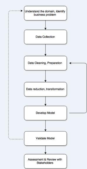
Figure: High Level Process Flow

•  Limitations

There are few limitations that this study has w.r.t data and the methodology that can be used.

• Due to time and cost constraints we could not deploy a primary source for data collection. We were not in a position to deploy primary pollution data collection by deploying near ground level monitoring system that are typically used in advanced countries for such Air Pollution studies. They help accurately capture the road level air pollution contributed maximum by the automobiles.
• Due to a very short window of 15 days for the Odd-Even Campaign, we had to live with a very small data size rendering the data unusable for any kind of rigorous statistical analysis.
• Since the Analysis & Models were built specifically for a particular location, the insights and the Models cannot be used for other locations in New Delhi or for other locations outside New Delhi.
• Since the Models were built on rather small data size (about a year), the models need to be strengthened with data of  at least another year or two. Till then, the Models are likely to work in a larger range,i.e. the variance is likely to be higher.

2. Data Description and Preparation

• Data Management

We have extracted data for a year across 23 variables. This was collected for about 4 centres in New Delhi, one centre in Bangalore and one in Chennai. Data was extracted from CPCB’s real Time Air Quality data monitoring application that is available on-line. We have also extracted Data for Odd-Even Pilot project (Phase I & II). This data covers 4/5 major pollutant parameters like SO2, NO2, CO, PM2.5 & PM 10. The data covers 15 days prior to The Pilot project and the 15 days after the Pilot project.

To derive a more accurate analysis of the pilot project, we have also collected data of social conversations that took place around the Odd-Even experiment (Phase II). We were able to collect nearly 1000 social mentions / conversation around this theme.

Table 1: Table showing List of Variables

• Data Quality

1. Pollutant level data for certain days was missing. Some days had data for only few of the variables. Data for the days where there was no data for key variables like PM 2.5, PM 10, NO2, SO2, CO were removed. There was no data available for few of the days on the source system itself.
2. Especially for Odd-Even Campaign, data was not reported for a few days (already on a short window of 15 days pre-campaign and 15 days post campaign) on the source system. After plummeting all such variables and observations, the data was merged.
3. There were 26 variables with 284 records for Anand Vihar; 289 records for Punjabi Bagh & 345 records for R.K. Puram

• Data Preparation

Variables Transformation

1. For building the Multiple Linear Regression Model, all the variables were transformed using logarithm
2. For Neural Network, no data transformation was

Missing values and Outliers

1. No specific missing value treatment was used
2. Days for which no data was available for the key variables, then that day’s record was removed from analysis
3. Only days where observations were recorded for the key variables were included in the analysis
4. Days in which outliers were present, the day’s record was removed from the data

3. Exploratory Data Analysis

The Exploratory Data Analysis is divided into three parts. They are:

1. Analyzing three cities air pollution data and check whether the number of vehicles & vehicle density have any impact on air pollution levels
2. Analyzing the data of three locations of New Delhi across various factors and find out any correlation exists between the factors
3. Analyzing the New Delhi Data to find out the impact of ‘Odd-Even’ experiment on the pollution levels (i.e. measured across 4/5 key parameters). Also, explore the social data and do a sentimental analysis for gauging people’s reaction to the experiment

• Analyzing the impact of Vehicle Density & Vehicle Population

Analyzing three City Air Pollution Data and check whether the number of vehicles and vehicle density have any impact on air pollution levels:

We used simple Graph to plot the Pollutant levels for PM2.5, SO2, NO2 & CO across New Delhi, Bangalore & Chennai. The Average Pollution levels of the Pollutants were mapped on X– axis and the Vehicle Density and the number of vehicles were plotted on the Y-axis.

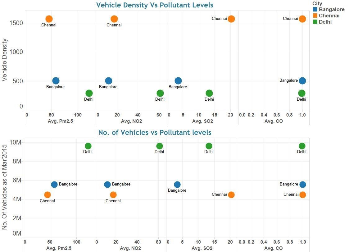
Figure: Graph showing Pollution Levels of 3 cities Vs Vehicle Density & Vehicle Population

• Insights

Vehicle density (measured as vehicles/km of road) does not have any impact on the air pollution. New Delhi has the least vehicle density amongst the three cities we have considered for the study, but the PM 2.5 levels are significantly higher in New Delhi as compared to Bangalore and Chennai. Though Chennai has the highest density of vehicles, but has a lower pollution levels for (PM 2.5)

1. If you consider the absolute vehicle population, then there seem to be a positive correlation between the number of vehicles and the air pollution levels of PM 2.5 & to a lesser extent on NO2.
2. CO levels does not seem to have any correlation with either vehicle density or with vehicle population as the levels of CO are almost at same levels across the 3 cities.
3. The result indicates the factors, other than vehicular pollution, contributing to the overall air pollution in the three cities are almost equal.
4. New Delhi has wide roads, so the vehicle density tends to get averaged out to a lower number.
5. But, there is a high probability that the vehicle density in many of the observatory locations are high and contributing to higher air pollution levels.

Identifying Patterns for Air Pollution in New Delhi

Our secondary research identified the three most polluted areas of New Delhi. They are Anand Vihar, R.K. Puram & Punjabi Bagh.

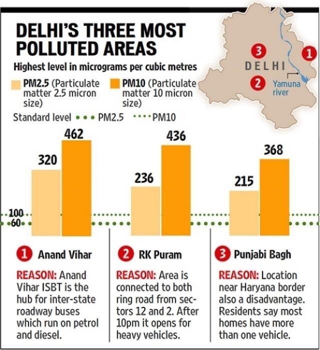
Figure: Chart showing the three most polluted areas of New Delhi.

•  Histogram for Various Pollutants

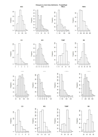
Histogram showing pollutant levels for each of the three locations – Anand Vihar, R.K.Puram & Punjabi Bagh

The histogram shows a few key attributes about the distribution of the different pollutants.

• Distribution is asymmetric – Left or right skewed
• Distribution is Unimodal in most pollutant data.
• There are some Outliers near the low and high ends

• Box Plot for Various Pollutants – All Locations

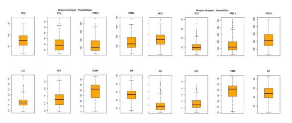
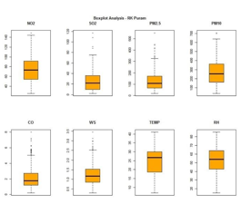
1. All the pollutants are almost at the same level in the 3 areas (Centres and spreads are equally likely for all 3 areas).
2. Indicating the areas between Anand Vihar, Punjabi Bagh and RK Puram are equally polluted.
3. The data has outliers caused by external factors and that needs to be investigated.

• Summary of Data for Key Variables for each Location
  

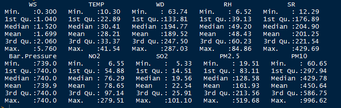
  Fig: Anand Vihar

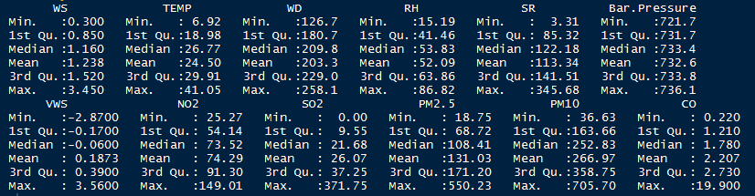
Fig: R.K.Puram

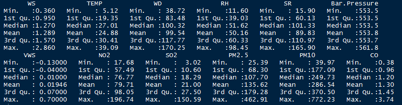
Fig: Punjabi Bagh

• Seasonality Analysis

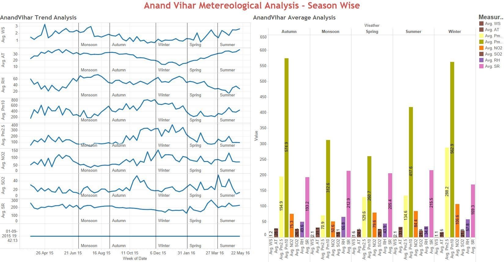
Fig:  Anand Vihar – Graph & Chart showing pollutant levels across seasons

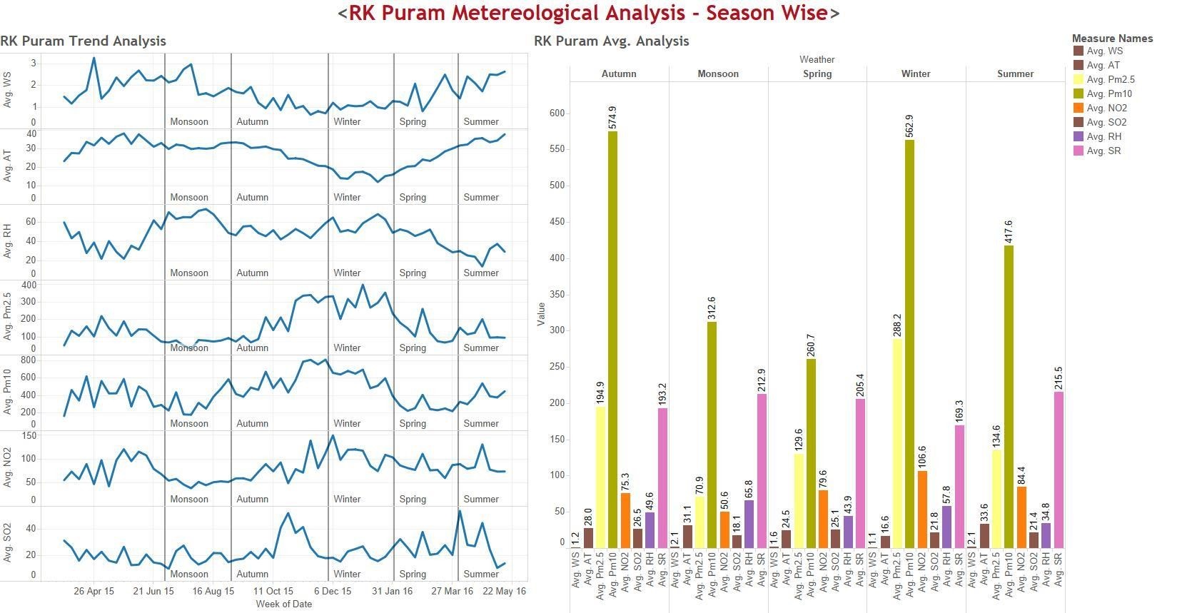
Figure:  R.K. Puram – Graph & Chart showing pollutant levels across seasons

Figure:  Punjabi Bagh – Graph & Chart showing pollutant levels across seasons

• Seasonality Analysis : Conclusion

1. Concentration of Particulate matter known as PM2.5 and PM10 are lower during Monsoon (July-August)
2. 5 and PM10 averages are exceeding its permissible values of 60 µg/m3 and 100 µg/m3 during WINTER (November-January) followed by AUTUMN (September-October), SUMMER (April-June) and to a lesser extend during SPRING (February-March)
3. Some kind of association between PM 2.5/PM 10 levels and Wind Speed as well as Temp can be seen in the graph
   • Relatively lower Pollution levels seem to be associated with higher Wind Speed
   • Very low Atmospheric Temperature is associated with relatively higher Pollution levels of PM 2.5/PM 10
4. Other pollutants data remains significantly same throughout the year except for NO2, peaks during winter and is at its lowest during monsoon

• Correlation Matrix & Analysis: Anand Vihar

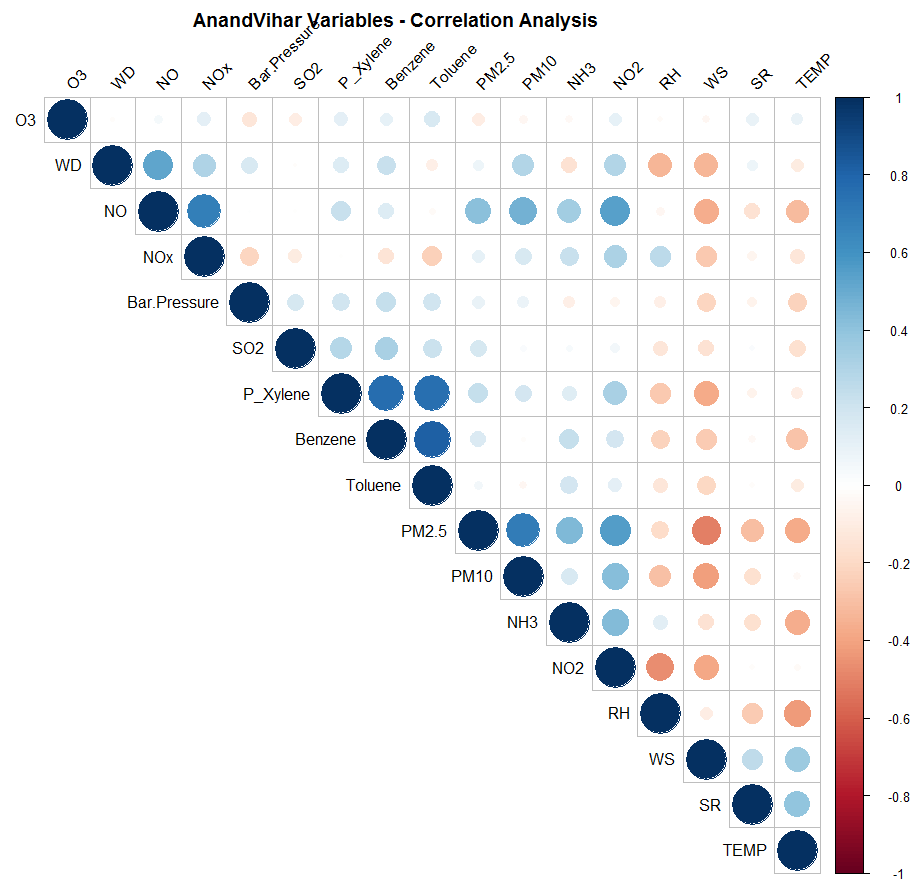
Figure: Correlation Matrix for Anand Vihar

Insights:

• PM 2.5 & 10 have a strong negative correlation with Wind Speed
• Temp has a negative correlation with PM 2.5, NH3 & Relative Humidity
• PM 2.5 also has a positive correlation with NO2
• Xylene, Toluene & Benzene are positively correlated with each other

• Correlation Matrix: Punjabi Bagh

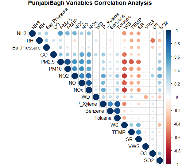
Figure: Correlation Matrix for Punjabi Bagh

Insights: 

• Wind Speed have a strong negative correlation with PM 2.5, 10, NO2, NO, CO, NH3 & NOx Wind Speed
• O3 has a strong negative correlation with RH
• Temp & SR also have some negative correlation with PM 2.5, PM 10, NO2, NH3
• Xylene, Toluene & Benzene are positively correlated with each other

• Correlation Matrix: R. K. Puram

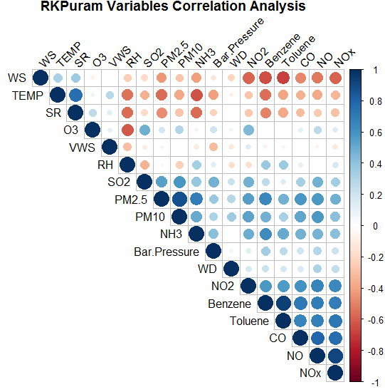
Figure: Correlation Matrix for R.K. Puram

Insights:

• PM 2.5, NO2, Benzene, Toluene, CO, NO have a strong negative correlation with Wind Speed and a negative correlation with Temp & SR
• O3 has a strong negative correlation with RH
• PM 2.5 also has a positive correlation with NO2, NO, CO, Benzene, Toluene
• Xylene, Toluene & Benzene are positively correlated with each other

4. Predictive Model Development

• Multiple Linear Regression Model (MLR) & Neural Network Model (NN)

The objective for the Predictive Model Development was to develop a model that can predict the next day’s level for key pollutants like PM 2.5, PM 10, SO2, CO etc.

The Model Development was done at multiple levels to arrive at a most suitable model. At first level we developed two sets of Model using Multi Linear Regression (MLR). The first one with the actual available variables. The second Model (MLR) was developed using one additional variable i.e. Previous Day’s level for that particular Pollutant (Dependent Variable).

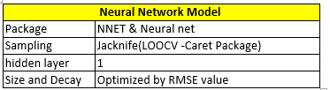
Then, at the second level we developed the Model using Neural Network (NN). Once again this was further divided in two parts. First with using all the available variables as they are. The second NN Model was developed using one additional variable i.e. Previous Day’s level for that particular Pollutant (Dependent Variable).

This Model building approach helped us with 4 sets of Model for each of the predictor variables, i.e, Key pollutants

The data for the modeling was split into two parts train & Test data. The Split of the data is as follows:

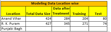
The following are the details for the Models:

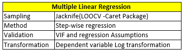
Since, the objective is to predict the next day’s value we have included the previous day’s level as Multiple Linear Regression which was run on Train data set using R package. Multi Linear Regression Model was used on Metrological variables like wind speed (WS), wind direction (WD), relative humidity (RH), solar radiation (SR) and temperature. The key pollutants like PM 2.5, PM 10, SO2, NO2, CO were kept as Dependent. Variables with low information value & high P-value were dropped. The resulting significant predictors, their p-values and the estimated signs for numeric predictors are shown in tables below.

Table showing Anand Vihar Air Pollution Predictive Model Results

Multiple Linear Regression Model Beta Coefficient Table

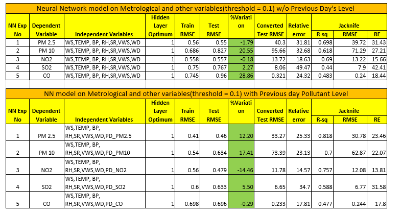
 Neural Network Model Results for w/o Previous Day’s and with PD’s

Inference:

• Almost 76.7% of the Variations in PM 2.5 seem to be explained by the MLR Model &73.9% by the Neural Network Model.

• NN gives a shade better RMSE value as compared to MLR. Model Fit seem to be significant for PM 5.

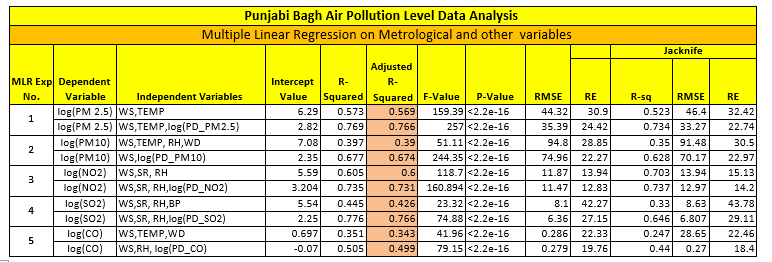
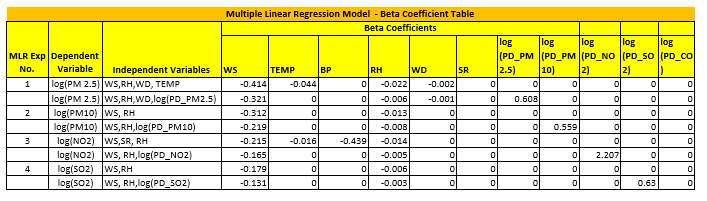
Table showing Punjabi Bagh Air Pollution Predictive Model Results

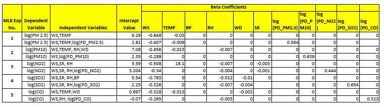
Multiple Linear Regression Model with Beta coefficients

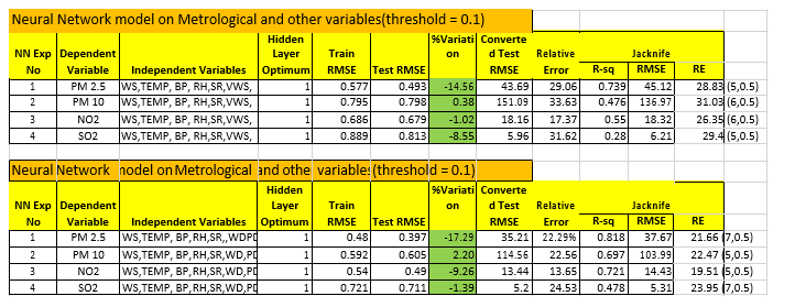
Neural Network Model without Previous Day’s value

Inference:

• 76% of the Variations in PM 2.5 seem to be explained by the MLR Model where as NN is able to explain 82% variation.
• NN gives a better RMSE value as compared to MLR with lower Relative Error %.
• Model Fit seem to be significant for PM 5.

• Model Fit Graphs

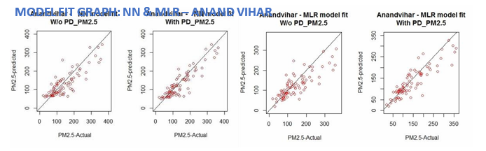
Fig: Anand Vihar – Comparative Model Fit graph for PM 2.5

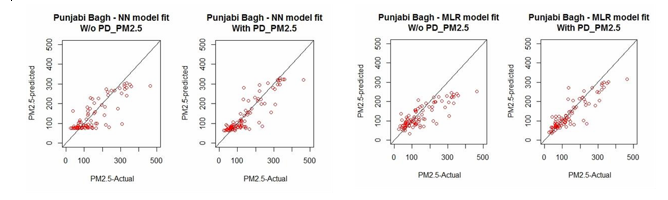
Fig: Punjabi Bagh – Comparative Model Fit Graph for PM 2.5

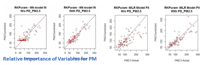
Fig: R.K. PURAM – Comparative Model Fit Graph for PM 2.5

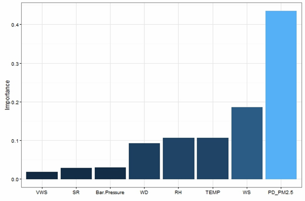
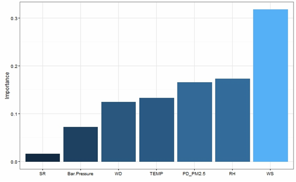
 Relative Importance Variables for the Three Locations

Inference: 

• Wind Speed is the most important variable for Punjabi Bag as well as Anand Vihar. It is the 2nd most important variable for R.K. Puram.
• Previous Day’s level is the second most important variable for PB and the most important variable for R.K Puram.
• Temp is the next important variable.

• Model Validation

We used Jackknife Validation Method for validating the 4 Models and their relative performance

We also used Root Mean Square Error (RMSE) Value method to validate and compare the relative performance of the 4 Models that we have developed.

We also performed the relative error check to validity of the model. The results of the three validations are presented in the table below.

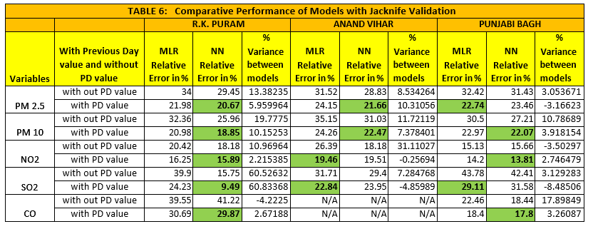
Inference:

• For all the predictor variables, Model built with Previous Day’s value provides the lowest Relative error. Across most of Predictor variable, Neural Network gives the lowest Relative Error in prediction. Only for Punjabi Bagh PM 2.5, SO2 & Anand Vihar’s NO2, SO2 MLR provides lower Relative error.

• Predictive Model Development Conclusions

1. Multiple Linear Regression Model is able to explain almost 76% of variations in PM 2.5 across all location. In comparison, Neural Network Model is able to explain up to 82% in R.K. Puram & Punjabi Bagh and to a lower 73.9% in Anand Vihar.
2. Neural Network overall is able to provide lower RMSE values for PM 2.5 & PM 10 across locations except for Punjabi Bagh (PM 2.5) where MLR gives a slightly lower RMSE
3. Wind Speed seem to be the most important independent variable followed by the Previous Day’s Value and
4. Model Fit seem to be significant for PM 2.5 for both the models across
5. Overall Neural Network Model was able to relatively perform better as compared to Multiple Linear Regression Model for predicting many pollutants across location.

Next Steps:

• Further strengthen the Model by including another 12-24 months of data. This will help further increase the accuracy of the
• There is some opportunity to do PCA Analysis, Factor Analysis and Discriminant Analysis to further separate the pollutant factors and identify the combinations of pollutants and its impact at each location. This could help the local administration to chart out a localized strategy for Pollution reduction.

5. ODD-EVEN Campaign

Analyzing the impact of the campaign on New Delhi’s air pollution levels

For the Odd-Even Campaign Analysis, we have taken 4 locations for consideration. They are:

• Anand Vihar
• Punjabi Bagh
• R. K. Puram
• Shadipur

The Key Air Pollutant levels were obtained for the 15 days prior to the Campaign and for the 15 days of the campaign period. For purpose of record, these days are:

Pre Campaign Period:                       1st  April 2016 to 14th April 2016

Campaign Period:                  15th  April 2016 to 30th April 2016

• Average Pollutant Level Analysis

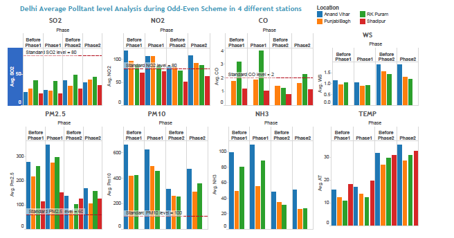
Fig: Average Pollutant Levels across 4 locations

Insights:

• PM 2.5, PM 10, CO & NO2 showed significant increase in levels during Odd-Even
• SO2 & NO3 showed marginal decline during Phase II
• All locations showed a drop in wind speed during the phase I & II of the ODD- EVEN Campaign

• Pollutant levels Trend Analysis

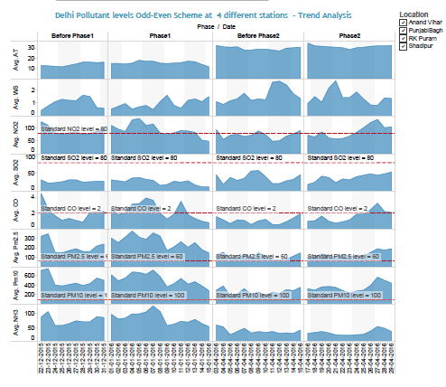
Fig: Pollution Level Trend Analysis Graph -All Locations combined

• Pollutant levels went up towards the end of Phase II accompanied by lower
• Pollutant levels dropped towards the end of Phase I accompanied by higher

• PM 2.5 & PM 10 Levels during Phase 2

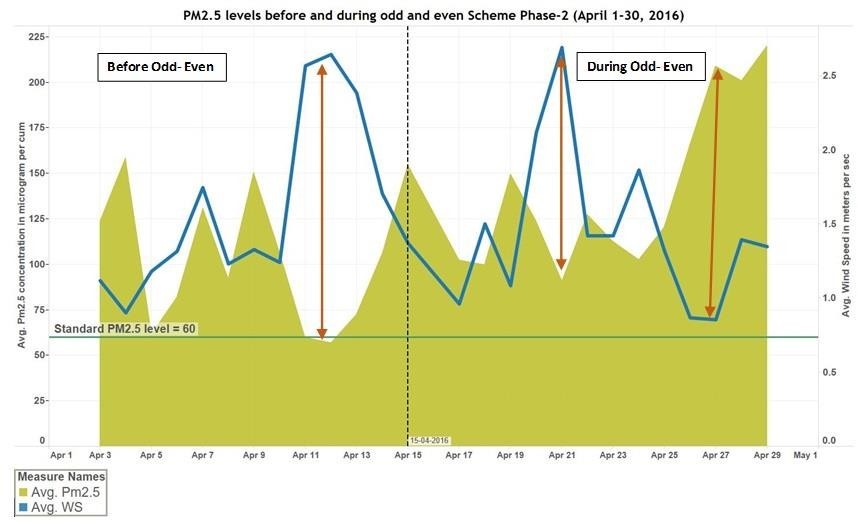
Figure (up) & (down): Graphs showing the PM 10 & PM 2.5 levels before and during Odd-Event Campaign (II)

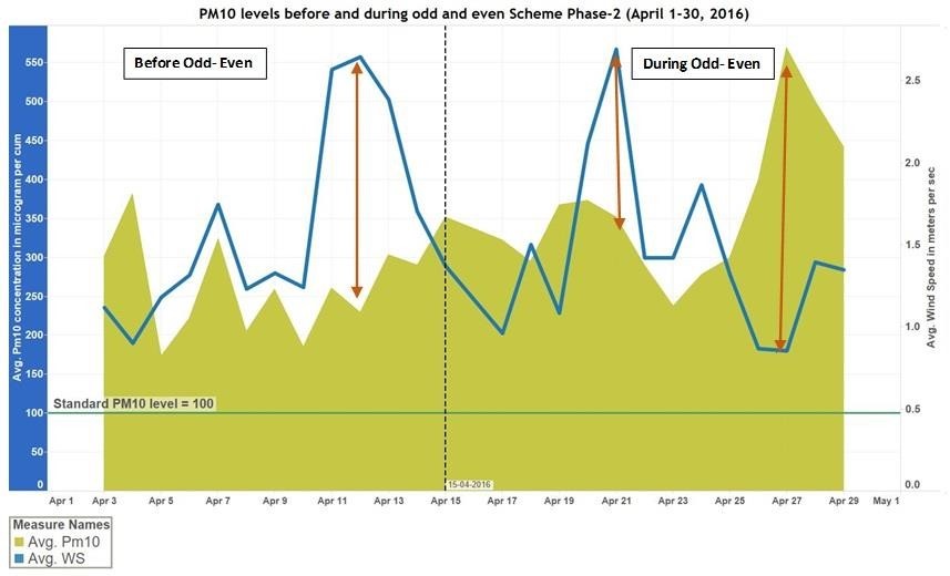
Insights:

• There is clear correlation between wind speed and PM 2.5 & PM 10
• Drop in wind Speed after 24th accompanied by spike in PM 2.5 levels

• ODD-EVEN Impact on Traffic (Cars)

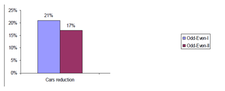
Fig: Impact on Number of Cars on the Road

Insights:

• Reduction in Cars on road between 8AM -8PM was 17% during Phase I, this dropped to 13% during phase II. Lower reduction rate attributed to: using 2nd car, taxis & CNG kit installation.

• Impact of Bio Mass Residual Burning on ODD-EVEN Campaign:

1. Satellite image substantiate impact of bio mass burning
2. 1st April image establish a near absence of any fire
3. 21st April image shows the start of the fire across Punjab, Haryana and Himalaya
4. 26th & 31st image establish the widespread fire phenomenon

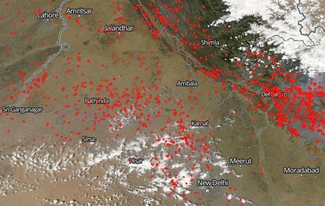
Fig: Picture showing the Bio Mass Burning across North India

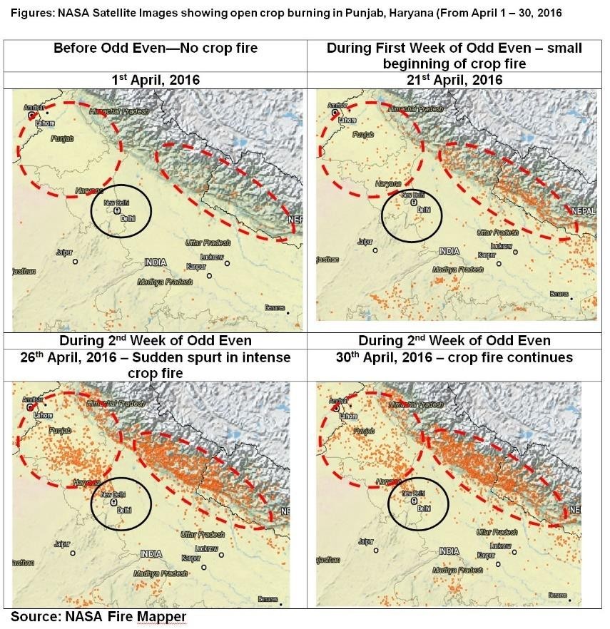
Fig: Picture showing the impact of Bio-Mass burning

• Satellite image showing the extent of Bio Mass burning immediately after the harvest.
• This year started around 19-21th
• Picture dated 26th April’16
• Setting of smog captured at the bottom

• Quantifying the Bio Mass Burning in India

Bio Mass Residual Burning – 2008-09 – State wise

1. 56% of PM 2.5 is contributed by the 4 neighbouring states of New Delhi, i.e, Haryana, Punjab, Rajasthan & Uttar Pradesh
2. Aided by wind speed and favourable wind direction the pollutants drift to New Delhi and compounding the air Pollution levels of the capital

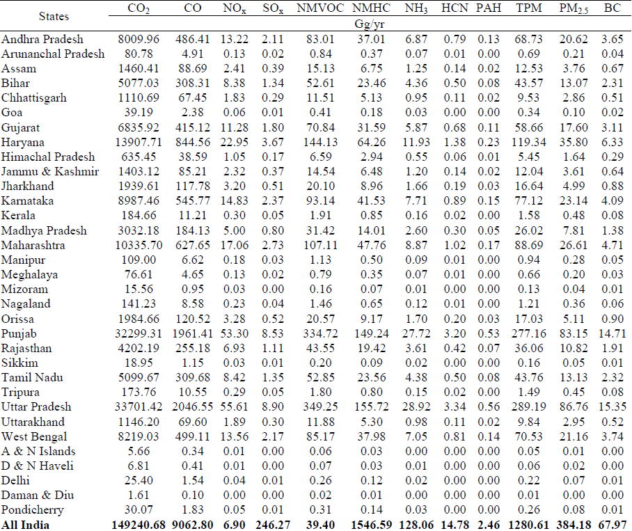
 Table showing the amount of Pollutant generated due to Bio-Mass burning across various States of India

• Text Mining of Tweets for Odd-Even Phase-II (April 15th 2016 – April 30th 2016) for Sentiment Analysis

1. Objective

As part of the study “Identifying Patterns in New Delhi’s Air Pollution”, text mining of tweets was undertaken to identify the sentiment of people towards Odd-Even Phase-II in New Delhi.

Odd-Even rule was levied by the Delhi Government to reduce air pollution in New Delhi. According to the rule, only the cars with odd  and even numbers were suppose to run on alternate days. The first trial period of this rule, i.e, Phase-I was applied from 1st January 2016 to 15th January 2016. The second trial period of this rule, i.e, Phase-II was applied from 15th  April 2016 to 30th April 2016.

During Phase-II the following vehicles were exempted from the rule:

1. Emergency services vehicles, such as, ambulances, fire engines, and those belonging to the hospitals, prisons, hearses, and law enforcement
2. SPG (Special Protection Group)
3. Vehicles with defence ministry numbers
4. Pilot Cars
5. Embassy Cars
6. Two-wheelers.

     2. Scope

The document describes the approach to mining of tweets for Odd-Even Phase-II.

• Mining of Tweets – Obtaining Tweets

The data pipeline built for mining of tweets is shown below:

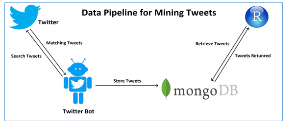
1. A twitter bot implemented in js is used for retrieving tweets from Twitter. The bot is configured to use the OAuth credentials received from the Twitter Developer account.
2. The bot is executed every day during the period of Odd-Even Phase-II.
3. The bot uses the Twitter search API to retrieve tweets filtered on ‘Odd-Even’.
4. The response of the Twitter search API is a JSON object which is then stored in MongoDB, which is a NoSQL
5. The twitter search APIs returns a maximum of 100 tweets for one
6. The response of Twitter search API contains tweets that were returned in an earlier search query thus resulting in duplication of
7. To resolve the duplication of tweets the ‘id’ (identifier) field of the tweet is, each tweet is identified by a unique ‘id’ which is returned in the response of the Twitter Search API. The ‘id’ is then used as a unique identifier rule set on the MongoDB collection, which ensures that only single copy of the tweet for a given ‘id’ is stored in MongoDB.
8. A total of 1172 unique tweets are collected during the Odd-Even Phase-II using this approach.

• Analysis of tweets

The tweets collected were analyzed using R through the following steps:

1. First using R package ‘rmongodb’ tweets are imported into R and converted into a data frame.
2. The ‘text’ column in the resulting data frame contains the tweet which is to be further analyzed.
3. The tweets in the ‘text’ column is then cleaned to remove punctuation characters, URLs etc.
4. The tweets are then normalized by converting all tweet to lower case
5. The cleansed tweets are then analyzed. The objective is to first create a word cloud and then analyze the sentiment of the cleansed
6. To create a word cloud R package ‘tm’ and ‘word cloud’ is
7. The tweets are first converted to ‘Corpus’ which is the data structure used for ‘tm’
8. As a result, all tweets are converted to
9. Then the stopwords are removed from these documents. Stopwords are common words that occur in a natural
10. After this the tweets in ‘Corpus’ is converted to ‘Term Document Matrix’. The ‘Term Document Matrix’ contains words as rows and documents(tweets) as columns. That is if a term (word) at the ith row of the matrix appears in a document (tweet) at the jth column of the matrix then the value 1 is stored at location [i][j] of the matrix else 0 is
11. Then using the ‘Tern Document Matrix’ term (word) frequencies are calculated which are then stored in a data frame with its associated word. Now we have each word with its frequency stored as a data
12. This is then visualized as a word cloud using the ‘wordcloud’
13. The cleansed tweets available at step ‘e’ is now analyzed for
14. Two kinds of scores are arrived at for each tweet. First scoring is based on emotional sentiments that a tweet has which can be – Anger, Anticipation, Disgust, Fear, Joy, Sadness, Surprise and Trust. The second type of score is based on polarity which indicates if a tweet carries a ‘positive’ sentiment or a ‘negative’
15. R packages ‘syuzhet’, ‘lubridate’, ‘scales’, ‘reshape2’, ‘dplyr’ are used to arrive at sentiment scores for each
16. To analyze the sentiment over time the time stamp associated with each time frame is
17. Each tweet has a timestamp which is specific to Twitter service. To process this in R these are converted into POSIX
18. Then R package ‘ggplot’ is used to visualize the sentiments over the period of Odd-Even Phase-II.

• Analysis Results

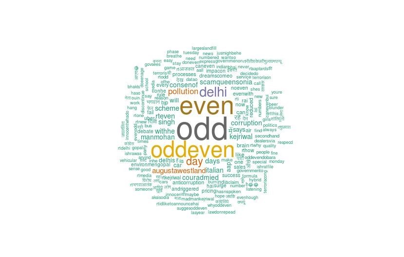
Word Cloud for Tweets Collected

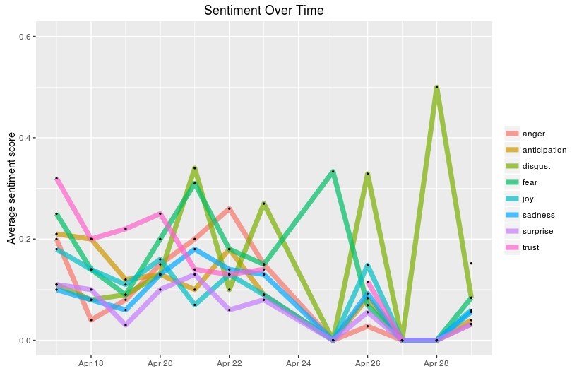
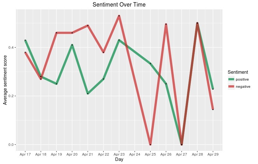
Fig: Sentiment Polarity of Tweets over Time

• Insights & Conclusions

• From the Sentiment analysis of the tweets collected for ‘Odd-Even’ Phase-II, it can be concluded that Twitterati largely holds negative sentiment towards this
• Twitterati mostly holds negative sentiment about Odd Even Phase 2 with increase in negative sentiments towards the end of the Odd Even Phase 2
• Campaign started with good sentiments like Trust, Joy, Unfortunately, negative sentiments like disgust took over from the second week onwards over-riding the positive sentiments.

1. Conclusions: Odd-Even Campaign

2. No apparent impact of ‘Odd-Even’ on the air pollution levels both during Phase I & Phase II
3. PM 2.5, PM 10, CO, NO2 & SO2 all showed increased levels during the Campaign periods as compared to the preceding 15
4. The Bio Mass (Crop Residual) burning in the neighbourhood states like Punjab, Haryana & Rajasthan also contributed to the increased levels of air pollutants post 19/20th April’16.
5. The average levels of Wind Speed went down during the Odd-Even Campaign Phase I & II contributing marginally to the increase in pollution
6. There is a strong possibility that any gains from Odd-Even scheme in terms of air quality levels were entirely eclipsed by “other sources of pollution”.
7. Some of the reasons for the lack of impact could be:
   • Vehicular pollution contributes only to 20% of Delhi’s air
   • Of this, only 13-14% is contributed by Cars (10% petrol and 4% diesel) a segment that was involved in the
   • Actual reduction in vehicle was only 13% during the campaign as compared to the normal
   • The other major contributing factors could be Road Dust -38%; domestic source-12% & Industrial pollutants-11%.
8. Any spike in any of these other factors could drastically alter the air pollution levels in Delhi.
9. Odd-Even Concept can work if it is not a for very long duration. It can work as an emergency short-term measure as done in Beijing for specific days when the pollution levels are expected / projected to exceed certain targeted levels.
10. If it is implemented at semi-permanent measure for longer duration, the impact is likely to be diluted as citizens are expected to circumvent the rule by opting for multiple car, two- wheelers, hire taxi, etc.

• Recommendations:

1. Introduce wet / machined vacuum sweeping of Roads
2. Evolve a system for reporting of garbage / municipal solid waste burning through a mobile based application and other social media platforms directly linked with control rooms
3. Set-up bio-mass based power generation units in the peripheral areas and neighboring states
4. Regulate carriage of construction materials in covered carriage
5. Take stringent action against open burning of bio-mass, tyres
6. Control dust pollution at construction sites with appropriate covers
7. Take steps for retrofitting the diesel vehicles with particulate filters
8. Extend LPG/PNG coverage to 100%. Follow it with a phase-out of charcoal and kerosene cooking in New Delhi
9. Engage Citizens actively and educate them on the need for participation as they are nor too happy with the Odd-Even Campaign. After the initial euphoria the sentiments about the Campaign turned

Strick Norms with ‘ALARM SYSTEM’ FOR Specific Decisive Interventions as illustrated here:

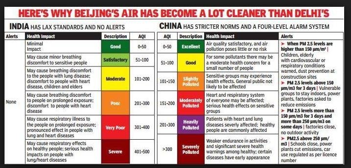
Fig: Chart showing Trigger Alarm and corrective action

End Notes

We hope this article was an enriching experience for you and provided you enough insights about the factors that can lead to rise in air pollution. so, watch out before we contribute to air pollution, knowingly or unknowingly. We thoroughly enjoyed working on this capstone project as part of our PGP-BABI program at Great Lakes. Our mentor guided us throughout and this project provided us immense learning.

Here is what our mentor, Mr. Jatinder Bedi, had to say about our Capstone Project, “Students wanted to do a typical legacy project in which they wanted to pick a dataset and run various Predictive models on top of it. I suggested them the idea of studying urban air pollution, a topic on which I was already working. I shared my thoughts and they picked up very smartly. The group had great energy to learn and was all willing to explore how concepts can be applied to real-world problems. It was an unsupervised study where we all learnt in every step. The project was a great showcase of how we can apply Analytics as a tool to understand problems around us and further take necessary steps to minimize the effects.”

Thanks to Dr. PKV for his consistent guidance and support. He has always been a great source of information for us.”

About the Authors

This article was contributed by Karthikeyan Gnanasekaran, Shrinivasabharathi Balasubramanian, Sankaranarayanan Mahadevan and Nagesh Shenoy M and the mentor Jatinder Bedi and was done as part of their capstone project. They were part of the Great Lakes PGPBABI program in Bangalore and finished their curriculum recently.

Got expertise in Business Intelligence  / Machine Learning / Big Data / Data Science? Showcase your knowledge and help Analytics Vidhya community by posting your blog.