Introduction
Lasso and ridge regression models work like magic in predicting the future using machine learning. Using these, businesses can predict future purchases and make better-informed decisions and future plans. In this article, I will explain everything you need to know about regression models and how to utilize them for prediction problems. We will thoroughly explore the fundamentals of linear, machine learning Lasso, and ridge regression models and understand their implementation in Python and R.
Learning Objectives
- Understand and implement linear regression techniques for predictive modeling.
- Understand regularization in regression models.
- Build Lasso, Ridge, and Elastic Net regression models.
Are you a beginner looking for a place to start your data science journey? Presenting a comprehensive course full of knowledge and data science learning curated just for you!

Table of contents
- Learning Example
- Simple Models for Prediction
- What Is Linear Regression?
- How to Find the Line of Best Fit for Lasso and ridge regression
- Gradient Descent
- Using Linear Regression for Prediction
- R Square and Adjusted R-Square
- Using All the Features for Prediction
- What Is Polynomial Regression?
- Bias and Variance in Lasso and lasso regression Regression Models
- Regularization of Models
- What Is Ridge Regression?
- What Is Lasso Regression?
- What Is Elastic Net Regression?
- Implementation in R
- Types of Regularization Techniques
- Frequently Asked Questions
Learning Example
Take a moment to list down all those factors you can think, on which the sales of a store will be dependent on Lasso and ridge regression model. For each factor create an hypothesis about why and how that factor would influence the sales of various products. For example – I expect the sales of products to depend on the location of the store, because the local residents in each area would have different lifestyle. The amount of bread a store will sell in Ahmedabad would be a fraction of similar store in Mumbai.
Similarly list down all possible factors you can think of.
Location of your shop, availability of the products, size of the shop, offers on the product, advertising done by a product, placement in the store could be some features on which your sales would depend on.
How many factors were you able to think of? If it is less than 15, give it more time and think again! A seasoned data scientist working on this problem would possibly think of tens and hundreds of such factors.
With that thought in mind, I am providing you with one such data set – The Big Mart Sales. In the data set, we have product wise Sales for Multiple outlets of a chain.
Let’s us take a snapshot of the dataset:

In the dataset of machine learning Lasso and ridge regression, we can see characteristics of the sold item (fat content, visibility, type, price) and some characteristics of the outlet (year of establishment, size, location, type) and the number of the items sold for that particular item. Let’s see if we can predict sales using these features.
Simple Models for Prediction
Let us start with ridge regression model making predictions using a few simple ways to start with. If I were to ask you, what could be the simplest way to predict the sales of an item, what would you say?
Model 1 – Mean sales
Even without any knowledge of machine learning, you can say that if you have to predict sales for an item – it would be the average over last few days . / months / weeks.
It is a good thought to start, but it also raises a question – how good is that model?
Turns out that there are various ways in which we can evaluate how good is our model. The most common way is Mean Squared Error. Let us understand how to measure it.
Prediction error
To evaluate how good is Lasso and ridge regression model, let us understand the impact of wrong predictions. If we predict sales to be higher than what they might be, the store will spend a lot of money making unnecessary arrangement which would lead to excess inventory. On the other side if I predict it too low, I will lose out on sales opportunity.
So, the simplest way of calculating error will be, to calculate the difference in the predicted and actual values. However, if we simply add them, they might cancel out, so we square these errors before adding. We also divide them by the number of data points to calculate a mean error since it should not be dependent on number of data points.

This is known as the mean squared error.
Here e1, e2 …. , en are the difference between the actual and the predicted values.
So, in our first machine learning Lasso and Ridge Regression model what would be the mean squared error? On predicting the mean for all the data points, we get a mean squared error = 29,11,799. Looks like huge error. May be its not so cool to simply predict the average value.
Let’s see if we can think of something to reduce the error. Here is a live coding window to predict target using mean.
Model 2 – Average Sales by Location
We know that location plays a vital role in the sales of an item. For example, let us say, sales of car would be much higher in Delhi than its sales in Varanasi. Therefore let us use the data of the column ‘Outlet_Location_Type’.
So basically, let us calculate the average sales for each location type and predict accordingly.
On predicting the same, we get mse = 28,75,386, which is less than our previous case. So we can notice that by using a characteristic[location], we have reduced the error.
Now, what if there are multiple features on which the sales would depend on. How would we predict sales using this information? Linear regression comes to our rescue.
What Is Linear Regression?
Linear regression is the simplest and most widely used statistical technique for predictive modeling. It basically gives us an equation, where we have our features as independent variables, on which our target variable [sales in our case] is dependent upon.
So what does the equation look like? Linear regression equation looks like this:

Here, we have Y as our dependent variable (Sales), X’s are the independent variables and all thetas are the coefficients. Coefficients are basically the weights assigned to the features, based on their importance. For example, if we believe that sales of an item would have higher dependency upon the type of location as compared to size of store, it means that sales in a tier 1 city would be more even if it is a smaller outlet than a tier 3 city in a bigger outlet. Therefore, coefficient of location type would be more than that of store size.
So, firstly let us try to understand linear regression with only one feature, i.e., only one independent variable. Therefore our equation becomes,

This equation is called a simple linear regression equation, which represents a straight line, where ‘Θ0’ is the intercept, ‘Θ1’ is the slope of the line. Take a look at the plot below between sales and MRP.

Surprisingly, we can see that sales of a product increases with increase in its MRP. Therefore the dotted red line represents our regression line or the line of best fit. But one question that arises is how you would find out this line?
How to Find the Line of Best Fit for Lasso and ridge regression
As you can see below there can be so many lines which can be used to estimate Sales according to their MRP. So how would you choose the best fit line or the regression line?

The main purpose of the best fit line is that our predicted values should be closer to our actual or the observed values, because there is no point in predicting values which are far away from the real values. In other words, we tend to minimize the difference between the values predicted by us and the observed values, and which is actually termed as error.
Graphical representation of error is as shown below
These errors are also called as residuals. The residuals are indicated by the vertical lines showing the difference between the predicted and actual value.

Okay, now we know that our main objective is to find out the error and minimize it. But before that, let’s think of how to deal with the first part, that is, to calculate the error. We already know that error is the difference between the value predicted by us and the observed value.
Three ways through which we can calculate error
- Sum of residuals (∑(Y – h(X))) – it might result in cancelling out of positive and negative errors.
- Sum of the absolute value of residuals (∑|Y-h(X)|) – absolute value would prevent cancellation of errors
- Sum of square of residuals ( ∑ (Y-h(X))2) – it’s the method mostly used in practice since here we penalize higher error value much more as compared to a smaller one, so that there is a significant difference between making big errors and small errors, which makes it easy to differentiate and select the best fit line.
Therefore, sum of squares of these residuals is denoted by:

where, h(x) is the value predicted by us, h(x) =Θ1*x +Θ0 , y is the actual values and m is the number of rows in the training set.
The cost Function
So let’s say, you increased the size of a particular shop, where you predicted that the sales would be higher. But despite increasing the size, the sales in that shop did not increase that much. So the cost applied in increasing the size of the shop, gave you negative results.
So, we need to minimize these costs. Therefore we introduce a cost function, which is basically used to define and measure the error of the model.

If you look at this equation carefully, it is just similar to sum of squared errors, with just a factor of 1/2m is multiplied in order to ease mathematics.
So in order to improve our prediction, we need to minimize the cost function. For this purpose we use the gradient descent algorithm. So let us understand how it works.
Gradient Descent
Let us consider an example, we need to find the minimum value of this equation,
Y= 5x + 4x^2. In mathematics, we simple take the derivative of this equation with respect to x, simply equate it to zero. This gives us the point where this equation is minimum. Therefore substituting that value can give us the minimum value of that equation.
Gradient descent works in a similar manner. It iteratively updates Θ, to find a point where the cost function would be minimum. If you wish to study gradient descent in depth, I would highly recommend going through this article.
Using Linear Regression for Prediction
Now let us consider using Linear Regression to predict Sales for our big mart sales problem.
Model 3 – Enter Linear Regression
From the previous case, we know that by using the right features would improve our accuracy. So now let us use two features, MRP and the store establishment year to estimate sales.
Now, let us built a linear regression model in python considering only these two features.
# importing basic libraries
import numpy as np
 import pandas as pd
from pandas import Series, DataFrame
from sklearn.model_selection import train_test_split
import test and train file
train = pd.read_csv('Train.csv')
test = pd.read_csv('test.csv')
# importing linear regressionfrom sklearn
from sklearn.linear_model import LinearRegression
lreg = LinearRegression()
splitting into training and cv for cross validation
X = train.loc[:,['Outlet_Establishment_Year','Item_MRP']]
x_train, x_cv, y_train, y_cv = train_test_split(X,train.Item_Outlet_Sales)
training the model
lreg.fit(x_train,y_train)
predicting on cv
pred = lreg.predict(x_cv)
calculating mse
mse = np.mean((pred - y_cv)**2)
In this case, we got mse = 19,10,586.53, which is much smaller than our model 2. Therefore predicting with the help of two features is much more accurate.
Let us take a look at the coefficients of this linear regression model.
# calculating coefficients
 coeff = DataFrame(x_train.columns)
 coeff['Coefficient Estimate'] = Series(lreg.coef_)
coeff
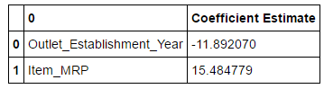
Therefore, we can see that MRP has a high coefficient, meaning items having higher prices have better sales.
R Square and Adjusted R-Square
How accurate do you think the model is? Do we have any evaluation metric, so that we can check this? Actually we have a quantity, known as R-Square.
R-Square: It determines how much of the total variation in Y (dependent variable) is explained by the variation in X (independent variable). Mathematically, it can be written as:

The value of R-square is always between 0 and 1, where 0 means that the model does not model explain any variability in the target variable (Y) and 1 meaning it explains full variability in the target variable.
Now let us check the r-square for the above model.
lreg.score(x_cv,y_cv)
 0.3287
In this case, R² is 32%, meaning, only 32% of variance in sales is explained by year of establishment and MRP. In other words, if you know year of establishment and the MRP, you’ll have 32% information to make an accurate prediction about its sales.
Now what would happen if I introduce one more feature in my model, will my model predict values more closely to its actual value? Will the value of R-Square increase?
Let us consider another case.
Model 4 – Linear regression with more variables
We learnt, by using two variables rather than one, we improved the ability to make accurate predictions about the item sales.
So, let us introduce another feature ‘weight’ in case 3. Now let’s build a regression model with these three features.
X = train.loc[:,['Outlet_Establishment_Year','Item_MRP','Item_Weight']]
splitting into training and cv for cross validation
x_train, x_cv, y_train, y_cv = train_test_split(X,train.Item_Outlet_Sales)
## training the model
lreg.fit(x_train,y_train)
ValueError: Input contains NaN, infinity or a value too large for dtype(‘float64’).
It produces an error, because item weights column have some missing values. So let us impute it with the mean of other non-null entries.
train['Item_Weight'].fillna((train['Item_Weight'].mean()), inplace=True)Let us try to run the model again.
training the model lreg.fit(x_train,y_train)
## splitting into training and cv for cross validation
x_train, x_cv, y_train, y_cv = train_test_split(X,train.Item_Outlet_Sales)
## training the model lreg.fit(x_train,y_train)
predicting on cv pred = lreg.predict(x_cv)
calculating mse
mse = np.mean((pred - y_cv)**2)
mse
1853431.59
## calculating coefficients
coeff = DataFrame(x_train.columns)
coeff['Coefficient Estimate'] = Series(lreg.coef_)

calculating r-square
lreg.score(x_cv,y_cv) 0.32942
Therefore we can see that the mse is further reduced. There is an increase in the value R-square, does it mean that the addition of item weight is useful for our model?
Adjusted R-square
The only drawback of R2 is that if new predictors (X) are added to our model, R2 only increases or remains constant but it never decreases. We can not judge that by increasing complexity of our model, are we making it more accurate?
That is why, we use “Adjusted R-Square”.
The Adjusted R-Square is the modified form of R-Square that has been adjusted for the number of predictors in the model. It incorporates model’s degree of freedom. The adjusted R-Square only increases if the new term improves the model accuracy.

where
R2 = Sample R square
p = Number of predictors
N = total sample size
Using All the Features for Prediction
Now let us built a model containing all the features. While building the regression models, I have only used continuous features. This is because we need to treat categorical variables differently before they can used in linear regression model. There are different techniques to treat them, here I have used one hot encoding(convert each class of a categorical variable as a feature). Other than that I have also imputed the missing values for outlet size.
Data pre-processing steps for regression model
# imputing missing values
train['Item_Visibility'] = train['Item_Visibility'].replace(0,np.mean(train['Item_Visibility']))
train['Outlet_Establishment_Year'] = 2013 - train['Outlet_Establishment_Year']
train['Outlet_Size'].fillna('Small',inplace=True)
# creating dummy variables to convert categorical into numeric values
mylist = list(train1.select_dtypes(include=['object']).columns)
dummies = pd.get_dummies(train[mylist], prefix= mylist)
train.drop(mylist, axis=1, inplace = True)
X = pd.concat([train,dummies], axis =1 )
Building the model
import numpy as np
import pandas as pd
from pandas import Series, DataFrame
import matplotlib.pyplot as plt
%matplotlib inline
train = pd.read_csv('training.csv')
test = pd.read_csv('testing.csv')
# importing linear regression
from sklearn from sklearn.linear_model import LinearRegression
lreg = LinearRegression()
# for cross validation
from sklearn.model_selection import train_test_split
X = train.drop('Item_Outlet_Sales',1)
x_train, x_cv, y_train, y_cv = train_test_split(X,train.Item_Outlet_Sales, test_size =0.3)
# training a linear regression model on train
lreg.fit(x_train,y_train)
# predicting on cv
pred_cv = lreg.predict(x_cv)
# calculating mse
mse = np.mean((pred_cv - y_cv)**2)
mse
1348171.96
# evaluation using r-square
lreg.score(x_cv,y_cv)
0.54831541460870059
Clearly, we can see that there is a great improvement in both mse and R-square, which means that our model now is able to predict much closer values to the actual values.
Selecting the right features for your model
When we have a high dimensional data set, it would be highly inefficient to use all the variables since some of them might be imparting redundant information. We would need to select the right set of variables which give us an accurate model as well as are able to explain the dependent variable well. There are multiple ways to select the right set of variables for the model. First among them would be the business understanding and domain knowledge. For instance while predicting sales we know that marketing efforts should impact positively towards sales and is an important feature in your model. We should also take care that the variables we’re selecting should not be correlated among themselves.
Instead of manually selecting the variables, we can automate this process by using forward or backward selection. Forward selection starts with most significant predictor in the model and adds variable for each step. Backward elimination starts with all predictors in the model and removes the least significant variable for each step. Selecting criteria can be set to any statistical measure like R-square, t-stat etc.
Interpretation of Regression Plots
Take a look at the residual vs fitted values plot.

residual plot
x_plot = plt.scatter(pred_cv, (pred_cv - y_cv), c='b')
plt.hlines(y=0, xmin= -1000, xmax=5000)
plt.title('Residual plot')
We can see a funnel like shape in the plot. This shape indicates Heteroskedasticity. The presence of non-constant variance in the error terms results in heteroskedasticity. We can clearly see that the variance of error terms(residuals) is not constant. Generally, non-constant variance arises in presence of outliers or extreme leverage values. These values get too much weight, thereby disproportionately influencing the model’s performance. When this phenomenon occurs, the confidence interval for out of sample prediction tends to be unrealistically wide or narrow.
We can easily check this by looking at residual vs fitted values plot. If heteroskedasticity exists, the plot would exhibit a funnel shape pattern as shown above. This indicates signs of non linearity in the data which has not been captured by the model. I would highly recommend going through this article for a detailed understanding of assumptions and interpretation of regression plots.
In order to capture this non-linear effects, we have another type of regression known as polynomial regression. So let us now understand it.
What Is Polynomial Regression?
Polynomial regression is another form of regression in which the maximum power of the independent variable is more than 1. In this regression technique, the best fit line is not a straight line instead it is in the form of a curve.
Quadratic regression, or regression with second order polynomial, is given by the following equation:
Y =Θ1 +Θ2*x +Θ3*x2
Now take a look at the plot given below.

Clearly the quadratic equation fits the data better than simple linear equation. In this case, what do you think will the R-square value of quadratic regression greater than simple linear regression? Definitely yes, because quadratic regression fits the data better than linear regression. While quadratic and cubic polynomials are common, but you can also add higher degree polynomials.
Below figure shows the behavior of a polynomial equation of degree 6.

So do you think it’s always better to use higher order polynomials to fit the data set. Sadly, no. Basically, we have created a model that fits our training data well but fails to estimate the real relationship among variables beyond the training set. Therefore our model performs poorly on the test data. This problem is called as over-fitting. We also say that the model has high variance and low bias.

Similarly, we have another problem called underfitting, it occurs when our model neither fits the training data nor generalizes on the new data.

Our model is underfit when we have high bias and low variance.
Bias and Variance in Lasso and lasso regression Regression Models
What does that bias and variance actually mean? Let us understand this by an example of archery targets.

Let’s say we have model which is very accurate, therefore the error of our model will be low, meaning a low bias and low variance as shown in first figure. All the data points fit within the bulls-eye. Similarly we can say that if the variance increases, the spread of our data point increases which results in less accurate prediction. And as the bias increases the error between our predicted value and the observed values increases.
Now how this bias and variance is balanced to have a perfect model? Take a look at the image below and try to understand.

As we add more and more parameters to our model, its complexity increases, which results in increasing variance and decreasing bias, i.e., overfitting. So we need to find out one optimum point in our model where the decrease in bias is equal to increase in variance. In practice, there is no analytical way to find this point. So how to deal with high variance or high bias?
To overcome underfitting or high bias, we can basically add new parameters to our model so that the model complexity increases, and thus reducing high bias.
Now, how can we overcome Overfitting for a regression model?
Two methods to overcome overfitting
- Reduce the model complexity
- Regularization
Here we would be discussing about Regularization in detail and how to use it to make your model more generalized.
Regularization of Models
You have your model ready, you have predicted your output. So why do you need to study regularization? Is it necessary?
Suppose you have taken part in a competition, and in that problem you need to predict a continuous variable. So you applied linear regression and predicted your output. Voila! You are on the leaderboard. But wait what you see is still there are many people above you on the leaderboard. But you did everything right then how is it possible?
“Everything should be made simple as possible, but not simpler – Albert Einstein”
What we did was simpler, everybody else did that, now let us look at making it simple. That is why, we will try to optimize our code with the help of regularization.
In regularization, what we do is normally we keep the same number of features, but reduce the magnitude of the coefficients j. How does reducing the coefficients will help us?
Let us take a look at the coefficients of feature in our above regression model.

checking the magnitude of coefficients
predictors = x_train.columns
coef = Series(lreg.coef_,predictors).sort_values()
coef.plot(kind='bar', title='Modal Coefficients')
We can see that coefficients of Outlet_Identifier_OUT027 and Outlet_Type_Supermarket_Type3(last 2) is much higher as compared to rest of the coefficients. Therefore the total sales of an item would be more driven by these two features.
How can we reduce the magnitude of coefficients in our model? For this purpose, we have different types of regression techniques which uses regularization to overcome this problem. So let us discuss them.
What Is Ridge Regression?
Let us first implement it on our above problem and check our results that whether it performs better than our linear regression model.
from sklearn.linear_model import Ridge
## training the model
ridgeReg = Ridge(alpha=0.05, normalize=True)
ridgeReg.fit(x_train,y_train)
pred = ridgeReg.predict(x_cv)
calculating mse
mse = np.mean((pred_cv - y_cv)**2)
mse 1348171.96 ## calculating score ridgeReg.score(x_cv,y_cv) 0.5691
So, we can see that there is a slight improvement in our model because the value of the R-Square has increased. Note that the value of alpha, which is a hyperparameter of Ridge, needs to be manually set as they are not automatically learned by the model.
Here we have consider alpha = 0.05. But let us consider different values of alpha and plot the coefficients for each case.


You can see that, as we increase the value of alpha, the magnitude of the coefficients decreases, where the values reaches to zero but not absolute zero.
But if you calculate R-square for each alpha, we will see that the value of R-square will be maximum at alpha=0.05. So we have to choose it wisely by iterating it through a range of values and using the one which gives us lowest error.
So, now you have an idea how to implement it but let us take a look at the mathematics side also. Till now our idea was to basically minimize the cost function, such that values predicted are much closer to the desired result.
Now take a look back again at the cost function for ridge regression.

Here, if you notice, we encounter an extra term known as the penalty term. The λ given here is actually denoted by the alpha parameter in the ridge function. By changing the values of alpha, we are essentially controlling the penalty term. The higher the values of alpha, the larger the penalty, resulting in the reduction of the magnitude of coefficients.
Important Points
- It shrinks the parameters, therefore it is mostly used to prevent multicollinearity.
- It reduces the model complexity by coefficient shrinkage.
- It uses L2 regularization technique. (which I will discussed later in this article)
Now let us consider another type of regression technique which also makes use of regularization.
What Is Lasso Regression?
LASSO (Least Absolute Shrinkage Selector Operator), is quite similar to ridge, but lets understand the difference them by implementing it in our big mart problem.
from sklearn.linear_model import Lasso
lassoReg = Lasso(alpha=0.3, normalize=True)
lassoReg.fit(x_train,y_train)
pred = lassoReg.predict(x_cv)
# calculating mse
mse = np.mean((pred_cv - y_cv)**2)
mse
1346205.82
lassoReg.score(x_cv,y_cv)
0.5720
As we can see that, both the mse and the value of R-square for our model has been increased. Therefore, lasso regression in machine learning model is predicting better than both linear and ridge.
Again lets change the value of alpha and see how does it affect the coefficients.

So, we can see that even at small values of alpha, the magnitude of coefficients have reduced a lot. By looking at the plots, can you figure a difference between ridge and lasso regression in machine learning?
We can see that as we increased the value of alpha, coefficients were approaching towards zero, but if you see in case of lasso, even at smaller alpha’s, our coefficients are reducing to absolute zeroes. Therefore, lasso selects the only some feature while reduces the coefficients of others to zero. This property is known as feature selection and which is absent in case of ridge.
Mathematics behind lasso regression in machine learning is quiet similar to that of ridge only difference being instead of adding squares of theta, we will add absolute value of Θ.

Here too, λ is the hypermeter, whose value is equal to the alpha in the Lasso function.
Important Points
- It uses L1 regularization technique (will be discussed later in this article)
- It is generally used when there are more features, as it automatically performs feature selection.
Now that you have a basic understanding of ridge and lasso regression, let’s think of an example where we have a large dataset, lets say it has 10,000 features. And we know that some of the independent features are correlated with other independent features. Then think, which regression would you use, Rigde or Lasso?
Let’s discuss it one by one. If we apply ridge regression to it, it will retain all of the features but will shrink the coefficients. But the problem is that model will still remain complex as there are 10,000 features, thus may lead to poor model performance.
Instead of ridge what if we apply lasso regression to this problem. The main problem with lasso regression is when we have correlated variables, it retains only one variable and sets other correlated variables to zero. That will possibly lead to some loss of information resulting in lower accuracy in our model.
Then what is the solution for this problem? Actually we have another type of regression, known as elastic net regression, which is basically a hybrid of ridge and lasso regression. So let’s try to understand it.
What Is Elastic Net Regression?
Before going into the theory part, let us implement this too in big mart sales problem. Will it perform better than ridge and lasso? Let’s check!
from sklearn.linear_model import ElasticNet
ENreg = ElasticNet(alpha=1, l1_ratio=0.5, normalize=False)
ENreg.fit(x_train,y_train)
pred_cv = ENreg.predict(x_cv)
#calculating mse
mse = np.mean((pred_cv - y_cv)**2)
mse 1773750.73
ENreg.score(x_cv,y_cv)
0.4504
So we get the value of R-Square, which is very less than both ridge and lasso. Can you think why? The reason behind this downfall is basically we didn’t have a large set of features. Elastic regression generally works well when we have a big dataset.
Note, here we had two parameters alpha and l1_ratio. First let’s discuss, what happens in elastic net, and how it is different from ridge and lasso regression.
Elastic net is basically a combination of both L1 and L2 regularization.
If you know elastic net, you can implement both Ridge and Lasso by tuning the parameters. So it uses both L1 and L2 penality term, therefore its equation look like as follows:

So how do we adjust the lambdas in order to control the L1 and L2 penalty term? Let us understand by an example. You are trying to catch a fish from a pond. And you only have a net, then what would you do? Will you randomly throw your net? No, you will actually wait until you see one fish swimming around, then you would throw the net in that direction to basically collect the entire group of fishes. Therefore even if they are correlated, we still want to look at their entire group.
Elastic lasso regression regression works in a similar way.
Let’ say, we have a bunch of correlated independent variables in a dataset, then elastic net will simply form a group consisting of these correlated variables. Now if any one of the variable of this group is a strong predictor (meaning having a strong relationship with dependent variable), then we will include the entire group in the model building, because omitting other variables (like what we did in lasso) might result in losing some information in terms of interpretation ability, leading to a poor model performance.
So, if you look at the code above, we need to define alpha and l1_ratio while defining the model. Alpha and l1_ratio are the parameters which you can set accordingly if you wish to control the L1 and L2 penalty separately. Actually, we have
Alpha = a + b and l1_ratio = a / (a+b)
where, a and b weights assigned to L1 and L2 term respectively. When we change the values of alpha and l1_ratio, we set a and b accordingly to control the trade-off between L1 and L2 as:
a * (L1 term) + b* (L2 term)
Let alpha (or a+b) = 1, and now consider the following cases
- If l1_ratio =1, therefore if we look at the formula of l1_ratio, we can see that l1_ratio can only be equal to 1 if a=1, which implies b=0. Therefore, it will be a lasso penalty.
- Similarly if l1_ratio = 0, implies a=0. Then the penalty will be a ridge penalty.
- For l1_ratio between 0 and 1, the penalty is the combination of ridge and lasso regression.
So let us adjust alpha and l1_ratio, and try to understand from the plots of coefficient given below.


Now, you have basic understanding about ridge, lasso and elasticnet regression. But during this, we came across two terms L1 and L2, which are basically two types of regularization. To sum up basically lasso and ridge are the direct application of L1 and L2 regularization respectively.
But if you still want to know, below I have explained the concept behind them, which is OPTIONAL but before that let us see the same implementation of above codes in R.
Implementation in R
Step 1: Linear regression with two variables “Item MRP” and “Item Establishment Year”.
Output
Call:
lm(formula = Y_train ~ Item_MRP + Outlet_Establishment_Year,
data = train_2)

Residuals:
Min 1Q Median 3Q Max
-4000.1 -769.4 -32.7 679.4 9286.7

Coefficients:
Estimate Std. Error t value Pr(>|t|)
(Intercept) 17491.6441 4328.9747 4.041 5.40e-05 ***
Item_MRP 15.9085 0.2909 54.680 < 2e-16 ***
Outlet_Establishment_Year -8.7808 2.1667 -4.053 5.13e-05 ***
---
Signif. codes: 0 ‘***’ 0.001 ‘**’ 0.01 ‘*’ 0.05 ‘.’ 0.1 ‘ ’ 1

Residual standard error: 1393 on 5953 degrees of freedom
Multiple R-squared: 0.3354, Adjusted R-squared: 0.3352
F-statistic: 1502 on 2 and 5953 DF, p-value: < 2.2e-16
Also, the value of r square is 0.3354391 and the MSE is 20,28,538.
Step 2: Linear regression with three variables “Item MRP”, “Item Establishment Year”, “Item Weight”.
Output
Call:
lm(formula = Y_train ~ Item_Weight + Item_MRP + Outlet_Establishment_Year,
data = train_2)

Residuals:
Min 1Q Median 3Q Max
-4000.7 -767.1 -33.2 680.8 9286.3

Coefficients:
Estimate Std. Error t value Pr(>|t|)
(Intercept) 17530.3653 4329.9774 4.049 5.22e-05 ***
Item_Weight -2.0914 4.2819 -0.488 0.625
Item_MRP 15.9128 0.2911 54.666 < 2e-16 ***
Outlet_Establishment_Year -8.7870 2.1669 -4.055 5.08e-05 ***
---
Signif. codes: 0 ‘***’ 0.001 ‘**’ 0.01 ‘*’ 0.05 ‘.’ 0.1 ‘ ’ 1

Residual standard error: 1393 on 5952 degrees of freedom
Multiple R-squared: 0.3355, Adjusted R-squared: 0.3351
F-statistic: 1002 on 3 and 5952 DF, p-value: < 2.2e-16
Also, the value of r square is 0.3354657 and the MSE is 20,28,692.
Step 3: Linear regression with all variables.
Output
Also, the value of r square is 0.3354657 and the MSE is 14,38,692.
Step 4: Implementation of Ridge regression
Output
 (Intercept) (Intercept) Item_Weight
-220.666749 0.000000 4.223814
Item_Fat_Contentlow fat Item_Fat_ContentLow Fat Item_Fat_Contentreg
450.322572 170.154291 -760.541684
Item_Fat_ContentRegular Item_Visibility Item_TypeBreads
-150.724872 589.452742 -80.478887
Item_TypeBreakfast Item_TypeCanned Item_TypeDairy
62.144579 638.515758 85.600397
Item_TypeFrozen Foods Item_TypeFruits and Vegetables Item_TypeHard Drinks
359.471616 -259.261220 -724.253049
Item_TypeHealth and Hygiene Item_TypeHousehold Item_TypeMeat
-127.436543 -197.964693 -62.876064
Item_TypeOthers Item_TypeSeafood Item_TypeSnack Foods
120.296577 -114.541586 140.058051
Item_TypeSoft Drinks Item_TypeStarchy Foods Item_MRP
-77.997959 1294.760824 9.841181
Outlet_IdentifierOUT013 Outlet_IdentifierOUT017 Outlet_IdentifierOUT018
20.653040 442.754542 252.958840
Outlet_IdentifierOUT019 Outlet_IdentifierOUT027 Outlet_IdentifierOUT035
-1044.171225 1031.745209 -213.353983
Outlet_IdentifierOUT045 Outlet_IdentifierOUT046 Outlet_IdentifierOUT049
-232.709629 249.947674 154.372830
Outlet_Establishment_Year Outlet_SizeHigh Outlet_SizeMedium
1.718906 18.560755 356.251406
Outlet_SizeSmall Outlet_Location_TypeTier 2 Outlet_Location_TypeTier 3
54.009414 50.276025 -369.417420
Outlet_TypeSupermarket Type1
649.021251
Step 5: Implementation of lasso regression
Output
 (Intercept) (Intercept) Item_Weight
550.39251 0.00000 0.00000
Item_Fat_Contentlow fat Item_Fat_ContentLow Fat Item_Fat_Contentreg
0.00000 22.67186 0.00000
Item_Fat_ContentRegular Item_Visibility Item_TypeBreads
0.00000 0.00000 0.00000
Item_TypeBreakfast Item_TypeCanned Item_TypeDairy
0.00000 0.00000 0.00000
Item_TypeFrozen Foods Item_TypeFruits and Vegetables Item_TypeHard Drinks
0.00000 -83.94379 0.00000
Item_TypeHealth and Hygiene Item_TypeHousehold Item_TypeMeat
0.00000 0.00000 0.00000
Item_TypeOthers Item_TypeSeafood Item_TypeSnack Foods
0.00000 0.00000 0.00000
Item_TypeSoft Drinks Item_TypeStarchy Foods Item_MRP
0.00000 0.00000 11.18735
Outlet_IdentifierOUT013 Outlet_IdentifierOUT017 Outlet_IdentifierOUT018
0.00000 0.00000 0.00000
Outlet_IdentifierOUT019 Outlet_IdentifierOUT027 Outlet_IdentifierOUT035
-580.02106 645.76539 0.00000
Outlet_IdentifierOUT045 Outlet_IdentifierOUT046 Outlet_IdentifierOUT049
0.00000 0.00000 0.00000
Outlet_Establishment_Year Outlet_SizeHigh Outlet_SizeMedium
0.00000 0.00000 260.63703
Outlet_SizeSmall Outlet_Location_TypeTier 2 Outlet_Location_TypeTier 3
0.00000 0.00000 -313.21402
Outlet_TypeSupermarket Type1
48.77124
For better understanding and more clarity on all the three types of regression, you can refer to this Free Course: Big Mart Sales In R.
Types of Regularization Techniques
Let’s recall, both in ridge and lasso regression we added a penalty term, but the term was different in both cases. In ridge, we used the squares of theta while in lasso we used absolute value of theta. So why these two only, can’t there be other possibilities?
Actually, there are different possible choices of regularization with different choices of order of the parameter in the regularization term, which is denoted by ![]() . This is more generally known as Lp regularizes.
. This is more generally known as Lp regularizes.
Let us try to visualize some by plotting them
For making visualization easy, let us plot them in 2D space. For that we suppose that we just have two parameters. Now, let’s say if p=1, we have term as ![]() . Can’t we plot this equation of line? Similarly plot for different values of p are given below.
. Can’t we plot this equation of line? Similarly plot for different values of p are given below.

In the above plots, axis denote the parameters(Θ1 and Θ2). Let us examine them one by one.
For p=0.5, we can only get large values of one parameter only if other parameter is too small. For p=1, we get sum of absolute values where the increase in one parameter Θ is exactly offset by the decrease in other.
Here p =2, we get a circle and for larger p values, it approaches a round square shape.
The two most commonly used regularization are in which we have p=1 and p=2, more commonly known as L1 and L2 regularization.
Look at the figure given below carefully.
The blue shape refers the regularization term and other shape present refers to our least square error (or data term).

The first figure is for L1 and the second one is for L2 regularization. The black point minimizes the least square error at that point, and we can see that it increases quadratically as we move from it, while the regularization term minimizes at the origin where all the parameters are zero.
Now the question is that at what point will our cost function be minimum? Since the terms are quadratically increasing, the sum of both terms will be minimized at the point where they first intersect.
Take a look at the L2 regularization curve. Since the shape formed by L2 regularizer is a circle, it increases quadratically as we move away from it. The L2 optimum(which is basically the intersection point) can fall on the axis lines only when the minimum MSE (mean square error or the black point in the figure) is also exactly on the axis.
But in case of L1, the L1 optimum can be on the axis line because its contour is sharp and therefore there are high chances of interaction point to fall on axis. Therefore it is possible to intersect on the axis line, even when minimum MSE is not on the axis. If the intersection point falls on the axes it is known as sparse.
Therefore, L1 provides some level of sparsity which makes our model more efficient to store and compute, and it can also help in checking the importance of features by exactly setting the unimportant features to zero.
Conclusion
I hope now you understand the science behind the linear regression and how to implement it and optimize it further to improve your model.
“Knowledge is the treasure and practice is the key to it”
Therefore, get your hands dirty by solving some problems. You can also start with the Big mart sales problem and try to improve your model with some feature engineering. If you face any difficulties while implementing it, feel free to write on our discussion portal.
Key Takeaways
- We now understand how to evaluate a linear regression model using R-squared and Adjusted R-squared values.
- We looked into the difference between Bias and Variance in regression models.
- We also learned to implement various regression models in R.
Frequently Asked Questions
Q1. What is the difference between LASSO and ridge regression?
A. LASSO regression performs feature selection by shrinking some coefficients to zero, whereas ridge regression shrinks coefficients but never reduces them to zero. Consequently, LASSO can produce sparse models, while ridge regression handles multicollinearity better.
Q2. What is Lasso Regression with an example?
A. Lasso Regression, or Least Absolute Shrinkage and Selection Operator, reduces less important feature coefficients to zero. For example, in predicting house prices, LASSO might eliminate irrelevant features like the number of windows, focusing only on significant ones like square footage.
Q3. What is the difference between ridge regression and linear regression?
A. Ridge regression, unlike linear regression, includes a penalty term that shrinks coefficients to prevent overfitting. As a result, ridge regression performs better when multicollinearity exists, whereas linear regression may overfit in such scenarios.
Q4. What is the full form of LASSO?
A. The full form of LASSO is Least Absolute Shrinkage and Selection Operator. This technique not only performs regression but also selects features by shrinking irrelevant coefficients to zero.
L1 regularizationL2 regularizationlasso regressionlinear regressionlive codingoverfittingPredictive modelingregressionregularizationridge regression
Shubham.jain Jain
27 Jun, 2024
I am currently pursing my B.Tech in Ceramic Engineering from IIT (B.H.U) Varanasi. I am an aspiring data scientist and a ML enthusiast. I am really passionate about changing the world by using artificial intelligence.


The way you explained it, mind blowing!!! Just hope I can reach your level :)
Thanks for the comment.
How to download The Big Mart Sales .data ?
You can find the train and test dataset from here : https://datahack.analyticsvidhya.com/contest/practice-problem-big-mart-sales-iii/
Very well explained Shubham. It was a wonderful read.
Thank you.
Thank you very much, Shubham. You could explain many subjects in just one article and so well. Well done. I just like to ask you if you mistakenly switched the place of independent and dependent in this paragraph, or I am confused about X and Y here: "R-Square: It determines how much of the total variation in Y (independent variable) is explained by the variation in X (dependent variable)."
Thanks for pointing out, it was a mistake from my side.
I liked the way you aproaches the contents. I will take a time to absorb the most of issues demonstrated, the theoretical aspects are a challenge for me at this moment, it is too much advanced for my basic statisticals knowledge
Can you tell what exactly happens when you # creating dummy variables to convert categorical into numeric values I try to translate your code to R, and I struggle a little bit there. Not sure what is the process, how dummy data look, and what are the final features you used.
Dummy encoding is used for categorical variables to convert each category into a separate column containing only 0 and 1, where 1 indicated its presence and 0 indicates its absence. For example, gender will contain two category, Male and female. So by dummy encoding them, you will create two separate variables, Var_M with values 1(Male) and 0 (no male) and Var_F with values 1 (female) and 0 (no female). You can use the "dummies" package for R for this. My final features includes all continuous variables and dummy variables for all categorical variables (make sure you drop the original column after encoding them), excluding Item_Identifier and Item_Outlet_Sales.
Hi, I am new to data science. I found the article quite interesting (theoretically). But when I try to implement things practically I have issues. May I know how was the mse ( mse = 28,75,386) calculated based on location?
I have basically calculated average sales for each location type and predicted the calculated values on the data based on their location type. Then mse was calculated using the formula given as: mse = np.mean((predicted_value - actual_value)**2)
Many complex concepts have been explained so nicely. Thank you very much for the article
Thank you.
Really very deep understanding article. Great work keep it up Surprising thing you gained this much knowledge while studying it self. This showing so much of your passion .
Thanks for the comment.
Thanks a lot Shubham for such a well explained article. This is one of the best article on linear regression I have come across which explains all possible concepts step by step like all dots connected together with simple explanation. I would really appreciate if you do same of kind of article on Logistic Regression. I look forward to it. Thanks again Shubham.
Glad that you liked the article. Sure, I will think of it. But we already have one article on logistic regression, if you wish, then you can check it out here: https://www.analyticsvidhya.com/blog/2015/11/beginners-guide-on-logistic-regression-in-r/
Nice work Shubham. Way to go man!
Thanks Pranjal.
Thank you so much team for nice explanation!
Thanks Vivek.
Great article Shubham!
Thanks Adity.
The article is just superb. My only curiosity about you...your interest into ML even though you are into ceramics engineering :) But again, the article is superb....i am reading it slowly with implementing each type of regression. I was working on the same data set prior to stumbling on your article. Helped a lot...thanks and cheers :)
Thanks abhishek. Glad you like the article. :)
Damn, that was an awesome read. Just perfect. Can you also do an article on how to do data analysis on terabytes of data? Like which server to buy, how to set it up, Apache spark, etc. I am eagerly waiting for that.
In STEP 7 Underneath building the model, you import a new data set with a different name (training instead of Train) is there another separate dataset?
No, it is the same dataset.
Thanks for the brilliant article Shubham! Gave me a holistic view of Linear Regression. Also, I have followed the concepts in the article and tried them at the Big Mart Problem. The code is documented here https://github.com/mohdsanadzakirizvi/Machine-Learning-Competitions/blob/master/bigmart/bigmart.md :)
Thanks Sanad. :)
Thanks Shubham,,, A very clean and neat explanation to beginners . I learnt about the regressions very well.. your way of presentation is awesome. Keep it up.. help us in understanding many such topics.
Very insightful article and nice explanation. However while trying to include all the features in the linear regression model (Section 7), R-sq increased only marginally to around 0.342...I have used the same code. Can you please help me figure out why I am getting this discrepancy?
This is one of the article which I would suggest to go through for any data scientist aspirant. Very well described on linear regression techniques.
nice article, you have exlplained the concepts in simplistic way.Thanks for the efforts.
Crystal Clear ,Must read ,Thanks Shubham
Thank you Shubham for the clear explanation and you have covered too much content in this article. Can you please try to give us the same on logistic regression, linear discriminant analysis, classification and regression tree, Random forest,svm etc.
Following is the code done in python 3.4. But I am getting a reduced Rsquared value as 0.3252 to 0.3251 after adding a feature. while i generate same set of train test set. Can you catch my mistake. Thanks for your time, also I appreciate your article. import numpy as np import os import matplotlib.pyplot as plt import pandas as pd from pandas import Series, DataFrame from sklearn.model_selection import train_test_split os.chdir('D:\HDFC') train = pd.read_csv('Train_set.csv') test = pd.read_csv('test_set.csv') from sklearn.linear_model import LinearRegression lreg=LinearRegression() ################################ SLR ############################### X=train.loc[:,['Outlet_Establishment_Year','Item_MRP']] x_train, x_cv, y_train, y_cv = train_test_split(X,train.Item_Outlet_Sales,random_state=300) lreg.fit(x_train,y_train) ##predicting on cv pred = lreg.predict(x_cv) ##calculating mse mse = np.mean((pred - y_cv)**2) # calculating coefficients coeff = DataFrame(x_train.columns) coeff['Coefficient Estimate'] = Series(lreg.coef_) coeff plt.scatter(x_cv.Item_MRP, y_cv, color='black') plt.plot(x_cv.Item_MRP, pred, color='blue', linewidth=3) ##plt.show() print(lreg.score(x_cv,y_cv)) ################################ MLR ############################ train['Item_Weight'].fillna((train['Item_Weight'].mean()), inplace=True) X = train.loc[:,['Outlet_Establishment_Year','Item_MRP','Item_Weight']] ##splitting into training and cv for cross validation x_train, x_cv, y_train, y_cv = train_test_split(X,train.Item_Outlet_Sales,random_state=300) train['Item_Weight'].fillna((train['Item_Weight'].mean()), inplace=True) ## training the model lreg.fit(x_train,y_train) pred = lreg.predict(x_cv) ##calculating mse ## calculating coefficients mse = np.mean((pred - y_cv)**2) coeff = DataFrame(x_train.columns) coeff['Coefficient Estimate'] = Series(lreg.coef_) print(lreg.score(x_cv,y_cv))
By far the best regression explanation so far. Never have I seen a textbook to explain why regression error is preferable to be considered as the sum of square of residuals and not the sum of absolute value of residuals. Thanks Shubham!
Is there any solved data set with multiple linear regression with issues of multi-col-linearity, heteroskedasticity, auto-correlation of error, over-fitting with their remedial measures?
Very good article! Could you just explain how to plot the figures where you show the values of the coefficients for Ridge and Lasso? Thank you very much Best Regards, Michael
I enjoyed this article better than rohit's 208
Could you please clarify on hetroskadacity in linear regression? Are non-linearity and hetroskadacity the same?In this article, they are treated as same,but in "Going Deeper into Regression Analysis with Assumptions, Plots & Solutions" they are termed as different.
Machaya Bro!!!! :)
Very appropriatle explained in consize and ideal manner! Thank You Sir
Hi Shubham, It is a good informative article! Can you please share the examples of python code for Polynomial Regression, adjusted-R square, Forward selection & Backward elimination?
Great introduction to the topic of shrinkage! Knowing there wasn't space to cover all the variants, one form of shrinkage that all data scientists should be aware of are random effects. More frequently used by statisticians in explanatory models, random effects have an application in predictive models in cases where data are clustered into multiple groups in which the response variables are correlated, and can be used in combination with other forms of penalization such as the lasso and ridge. For example, let's say you have to predict the future medical cost of the next insurance claim per member given a dataset containing 10 million past claim records for 1 million members and 10 claims per member, We'll assume the 10 claim amounts per member are approximately normally distributed. Rather than including 1 million categorical variables to account for member-level effects, a better predictive model would include a single random effect. Furthermore, if the members themselves are clustered into other categories, such as hospital, another level of random effects can be introduced in a hierarchical model.
Beautiful explanation, quite flawless !! Easy to understand. I wish to have a teacher like you throughout my journey to be a 'true' data scientist.
Exceptional article, really.Looking forward to your more articles Shubham
Exceptional article
A perfect article on regression which most of the books failed to explain it. I read this topic on couple of neural network books but it was very untidily portrayed. The X-factor of this article was the Big mart example you choosed. Clearing all my doubts with ease. Just great! Thank you. And would love to read more articles and such awesome explanations on ML.
Very well explained!
Very well explained. Superb. If you are ok can you tell us what is your source of information. I would really like to follow it.
Finally understood how regularization works! Thanks a lot!
Great article, thanks so much!
Hi Dina, Glad you liked it!
Extremely informative write-up!! The figures are so self explanatory too! Thank you!
Hi Roshni Glad you found this helpful!
This was really good. You covered everything and its really helpful.
Hi Chirag, Thank you for the feedback.Glad you found this useful!
you really did a great job thanks . Can you also do an article on dimension reduction?
Hi Subham, I guess the statement "How many factors were you able to think of? If it is less than 15, think again! A data scientist working on this problem would possibly think of hundreds of such factor." It is rude to me and I am sorry to say because I felt its offensive to me as you cannot just say every data scientist could possibly think like how you think
Hi AB, Feature engineering is a very difficult process to grasp. I am sure the author only wanted to convey that it is important to create more than 15-20 features, rather than discourage the readers. I agree that this could have been conveyed in a better way. We will update the article accordingly. Thank you for your feedback.
Hi Sir, Please share the data. On the given link i am not able to get the data set. And without data set how would i practice . your article is great. Thanks.
Hi Shubham, Thanks for the article, its quite informative. Would it be possible for you to share references you have gone through while working on this article
Your explaination is really very wonderful. Language is easy to understand. Explained really well n in simple way. Finally beatiful quote written '“Knowledge is the treasure and practice is the key to it”. Therefore, get your hands dirty by solving some problems. That was inspiring. Thanku so much all the best for ur future in AI. Thanku
Beautiful Greetings from your junior at IITBHU
when I click on the link of Dataset it redirect to another page but I did not find any dataset. please provide valid link in the article. Thanks
Jain Elastic, offered by Jain Narrow Fabrics, is a game-changer in elastic materials. With a reputation for quality and innovation, Jain Narrow Fabrics has once again delivered a product that exceeds expectations. Whether in the fashion industry, medical field, or any other sector that relies on elastic materials, Jain Elastic is the go-to choice. Its durability, stretchability, and versatility make it indispensable in various applications. Trust Jain Narrow Fabrics for all your elastic needs; they've proven time and again to be leaders in the industry. #JainElastic #InnovationInElasticMaterials #JainNarrowFabrics