An Overview of Regularization in Deep Learning (with Python code)
Introduction
One of the most common challenges encountered by data science professionals is the issue of overfitting. Have you ever experienced a scenario where your model excelled on the training data but struggled to make accurate predictions on unseen test data? Or perhaps you found yourself at the pinnacle of a competition’s public leaderboard, only to plummet in the final rankings? If so, this article is tailored to address your concerns by exploring techniques such as regularization in deep learning, alongside the essential concepts of bagging, boosting, and stacking in ensemble learning.
Avoiding overfitting can single-handedly improve our model’s performance.

In this article, we will understand the concept of overfitting and how regularization in deep learning helps in overcoming the same problem. We will then look at a few different regularization techniques and take a case study in python to further solidify these concepts.
Note: This article assumes that you have basic knowledge of neural networks and their implementation in Keras. If not, you can refer to the below articles first:
- Fundamentals of Deep Learning – Starting with Artificial Neural Network
- Tutorial: Optimizing Neural Networks using Keras (with Image recognition case study)
Table of contents
What is Regularization?
Regularization is a technique used in machine learning and deep learning to prevent overfitting and improve the generalization performance of a model. It involves adding a penalty term to the loss function during training.
This penalty discourages the model from becoming too complex or having large parameter values, which helps in controlling the model’s ability to fit noise in the training data. Regularization in deep learning methods include L1 and L2 regularization, dropout, early stopping, and more. By applying regularization, models become more robust and better at making accurate predictions on unseen data.
Before we deep dive into the topic, take a look at this image:
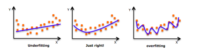
Have you seen this image before? As we move towards the right in this image, our model tries to learn too well the details and the noise from the training data, which ultimately results in poor performance on the unseen data.
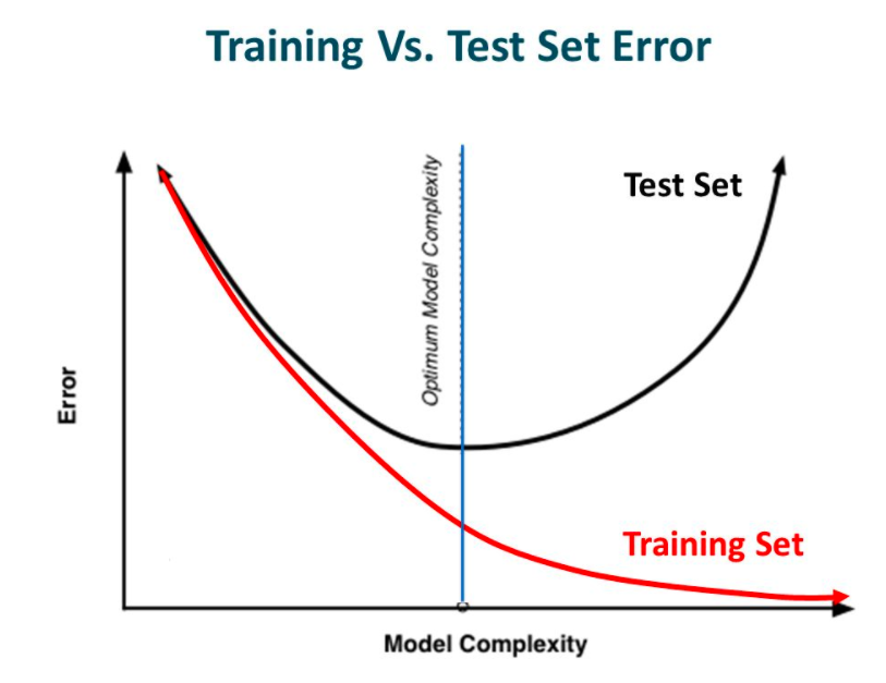
In other words, while going towards the right, the complexity of the model increases such that the training error reduces but the testing error doesn’t. This is shown in the image below.
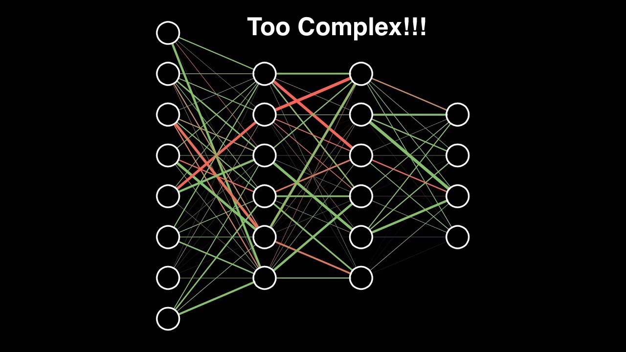
If you’ve built a neural network before, you know how complex they are. This makes them more prone to overfitting.
Regularization is a technique which makes slight modifications to the learning algorithm such that the model generalizes better. This in turn improves the model’s performance on the unseen data as well.
How does Regularization help reduce Overfitting?
Let’s consider a neural network which is overfitting on the training data as shown in the image below.
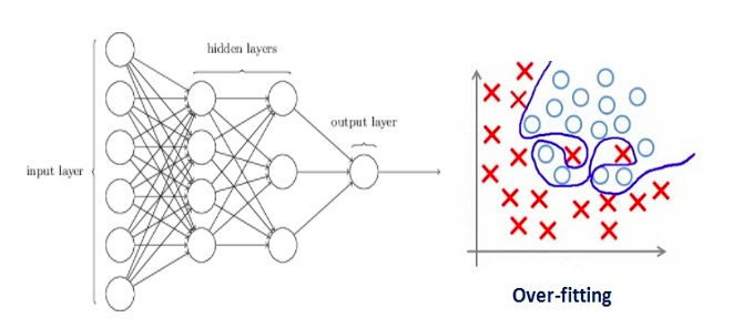
If you have studied the concept of regularization in machine learning, you will have a fair idea that regularization penalizes the coefficients. In deep learning, it actually penalizes the weight matrices of the nodes.
Assume that our regularization coefficient is so high that some of the weight matrices are nearly equal to zero.
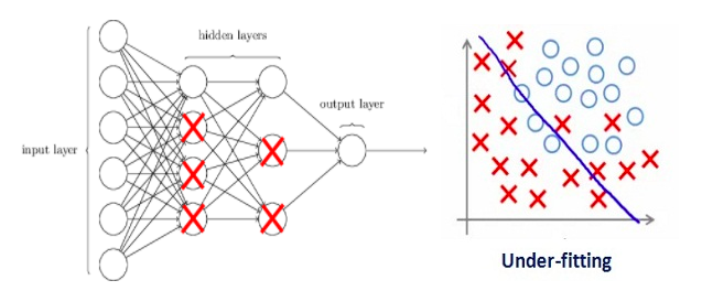
This will result in a much simpler linear network and slight underfitting of the training data.
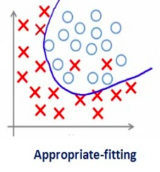
Such a large value of the regularization coefficient is not that useful. We need to optimize the value of regularization coefficient in order to obtain a well-fitted model as shown in the image below.
Different Regularization Techniques in Deep Learning
Now that we have an understanding of how regularization helps in reducing overfitting, we’ll learn a few different techniques in order to apply regularization in deep learning.
L2&L1 regularization
L1 and L2 are the most common types of regularization. These update the general cost function by adding another term known as the regularization term.
- Cost function = Loss (say, binary cross entropy) + Regularization term
Due to the addition of this regularization term, the values of weight matrices decrease because it assumes that a neural network with smaller weight matrices leads to simpler models. Therefore, it will also reduce overfitting to quite an extent.
However, this regularization term differs in L1 and L2.
In L2, we have:
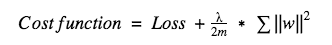
Here, lambda is the regularization parameter. It is the hyperparameter whose value is optimized for better results. L2 regularization is also known as weight decay as it forces the weights to decay towards zero (but not exactly zero).
In L1, we have:
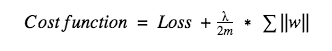
In this, we penalize the absolute value of the weights. Unlike L2, the weights may be reduced to zero here. Hence, it is very useful when we are trying to compress our model. Otherwise, we usually prefer L2 over it.
In keras, we can directly apply regularization to any layer using the regularizers.
Below is the sample code to apply L2 regularization to a Dense layer.
from keras import regularizers
model.add(Dense(64, input_dim=64,
                kernel_regularizer=regularizers.l2(0.01)
Note: Here the value 0.01 is the value of regularization parameter, i.e., lambda, which we need to optimize further. We can optimize it using the grid-search method.
Similarly, we can also apply L1 regularization. We will look at this in more detail in a case study later in this article.
Dropout
This is the one of the most interesting types of regularization techniques. It also produces very good results and is consequently the most frequently used regularization technique in the field of deep learning.
To understand dropout, let’s say our neural network structure is akin to the one shown below:
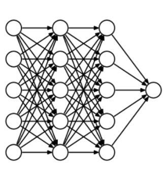
So what does dropout do? At every iteration, it randomly selects some nodes and removes them along with all of their incoming and outgoing connections as shown below.
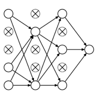
So each iteration has a different set of nodes and this results in a different set of outputs. It can also be thought of as an ensemble technique in machine learning.
Ensemble models usually perform better than a single model as they capture more randomness. Similarly, dropout also performs better than a normal neural network model.
This probability of choosing how many nodes should be dropped is the hyperparameter of the dropout function. As seen in the image above, dropout can be applied to both the hidden layers as well as the input layers.
Due to these reasons, dropout is usually preferred when we have a large neural network structure in order to introduce more randomness.
In keras, we can implement dropout using the keras core layer. Below is the python code for it:
from keras.layers.core import Dropout

model = Sequential([
 Dense(output_dim=hidden1_num_units, input_dim=input_num_units, activation='relu'),
 Dropout(0.25),

Dense(output_dim=output_num_units, input_dim=hidden5_num_units, activation='softmax'),
 ])
As you can see, we have defined 0.25 as the probability of dropping. We can tune it further for better results using the grid search method.
Data Augmentation
The simplest way to reduce overfitting is to increase the size of the training data. In machine learning, we were not able to increase the size of training data as the labeled data was too costly.
But, now let’s consider we are dealing with images. In this case, there are a few ways of increasing the size of the training data – rotating the image, flipping, scaling, shifting, etc. In the below image, some transformation has been done on the handwritten digits dataset.
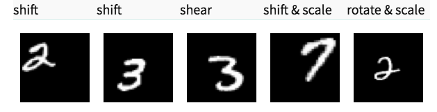
This technique is known as data augmentation. This usually provides a big leap in improving the accuracy of the model. It can be considered as a mandatory trick in order to improve our predictions.
In keras, we can perform all of these transformations using ImageDataGenerator. It has a big list of arguments which you you can use to pre-process your training data.
Below is the sample code to implement it.
from keras.preprocessing.image import ImageDataGenerator
datagen = ImageDataGenerator(horizontal flip=True)
datagen.fit(train)
Early stopping
Early stopping is a kind of cross-validation strategy where we keep one part of the training set as the validation set. When we see that the performance on the validation set is getting worse, we immediately stop the training on the model. This is known as early stopping.
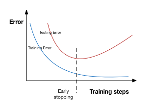
In the above image, we will stop training at the dotted line since after that our model will start overfitting on the training data.
In keras, we can apply early stopping using the callbacks function. Below is the sample code for it.
from keras.callbacks import EarlyStopping

EarlyStopping(monitor='val_err', patience=5)
Here, monitor denotes the quantity that needs to be monitored and ‘val_err’ denotes the validation error.
Patience denotes the number of epochs with no further improvement after which the training will be stopped. For better understanding, let’s take a look at the above image again. After the dotted line, each epoch will result in a higher value of validation error. Therefore, 5 epochs after the dotted line (since our patience is equal to 5), our model will stop because no further improvement is seen.
Note: It may be possible that after 5 epochs (this is the value defined for patience in general), the model starts improving again and the validation error starts decreasing as well. Therefore, we need to take extra care while tuning this hyperparameter.
A case study on MNIST data with keras
By this point, you should have a theoretical understanding of the different techniques we have gone through. We will now apply this knowledge to our deep learning practice problem – Identify the digits. Once you have downloaded the dataset, start following the below code! First, we’ll import some of the basic libraries.
%pylab inline
import numpy as np
import pandas as pd
from scipy.misc import imread
from sklearn.metrics import accuracy_score
from matplotlib import pyplot
import tensorflow as tf
import keras
# To stop potential randomness
seed = 128
rng = np.random.RandomState(seed)
Now, let’s load the dataset.
root_dir = os.path.abspath('/Users/shubhamjain/Downloads/AV/identify the digits/')
data_dir = os.path.join(root_dir, 'data')
sub_dir = os.path.join(root_dir, 'sub')
## reading train file only
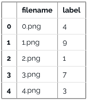
train = pd.read_csv(os.path.join(data_dir, 'Train', 'train.csv'))
train.head()
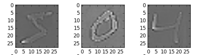
Take a look at some of our images now.
img_name = rng.choice(train.filename)

filepath = os.path.join(data_dir, 'Train', 'Images', 'train', img_name)

img = imread(filepath, flatten=True)

pylab.imshow(img, cmap='gray')
pylab.axis('off')
pylab.show()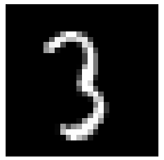
#storing images in numpy arrays
temp = []
for img_name in train.filename:
 image_path = os.path.join(data_dir, 'Train', 'Images', 'train', img_name)
 img = imread(image_path, flatten=True)
 img = img.astype('float32')
 temp.append(img)

x_train = np.stack(temp)

x_train /= 255.0
x_train = x_train.reshape(-1, 784).astype('float32')

y_train = keras.utils.np_utils.to_categorical(train.label.values)
Create a validation dataset, in order to optimize our model for better scores. We will go with a 70:30 train and validation dataset ratio.
split_size = int(x_train.shape[0]*0.7)

x_train, x_test = x_train[:split_size], x_train[split_size:]
y_train, y_test = y_train[:split_size], y_train[split_size:]
First, let’s start with building a simple neural network with 5 hidden layers, each having 500 nodes.
# import keras modules
from keras.models import Sequential
from keras.layers import Dense

# define vars
input_num_units = 784
hidden1_num_units = 500
hidden2_num_units = 500
hidden3_num_units = 500
hidden4_num_units = 500
hidden5_num_units = 500
output_num_units = 10

epochs = 10
batch_size = 128

model = Sequential([
 Dense(output_dim=hidden1_num_units, input_dim=input_num_units, activation='relu'),
 Dense(output_dim=hidden2_num_units, input_dim=hidden1_num_units, activation='relu'),
 Dense(output_dim=hidden3_num_units, input_dim=hidden2_num_units, activation='relu'),
 Dense(output_dim=hidden4_num_units, input_dim=hidden3_num_units, activation='relu'),
 Dense(output_dim=hidden5_num_units, input_dim=hidden4_num_units, activation='relu'),

Dense(output_dim=output_num_units, input_dim=hidden5_num_units, activation='softmax'),
 ])
Evaluating the Model
Note that we are just running it for 10 epochs. Let’s quickly check the performance of our model.
model.compile(loss='categorical_crossentropy', optimizer='adam', metrics=['accuracy'])

trained_model_5d = model.fit(x_train, y_train, nb_epoch=epochs, batch_size=batch_size, validation_data=(x_test, y_test))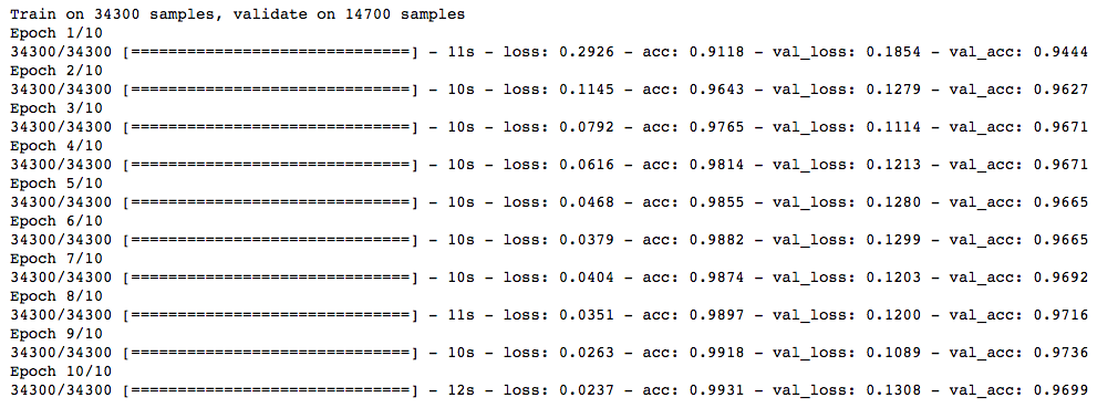
Now, let’s try the L2 regularizer over it and check whether it gives better results than a simple neural network model.
from keras import regularizers

model = Sequential([
 Dense(output_dim=hidden1_num_units, input_dim=input_num_units, activation='relu',
 kernel_regularizer=regularizers.l2(0.0001)),
 Dense(output_dim=hidden2_num_units, input_dim=hidden1_num_units, activation='relu',
 kernel_regularizer=regularizers.l2(0.0001)),
 Dense(output_dim=hidden3_num_units, input_dim=hidden2_num_units, activation='relu',
 kernel_regularizer=regularizers.l2(0.0001)),
 Dense(output_dim=hidden4_num_units, input_dim=hidden3_num_units, activation='relu',
 kernel_regularizer=regularizers.l2(0.0001)),
 Dense(output_dim=hidden5_num_units, input_dim=hidden4_num_units, activation='relu',
 kernel_regularizer=regularizers.l2(0.0001)),

Dense(output_dim=output_num_units, input_dim=hidden5_num_units, activation='softmax'),
 ])
model.compile(loss='categorical_crossentropy', optimizer='adam', metrics=['accuracy'])
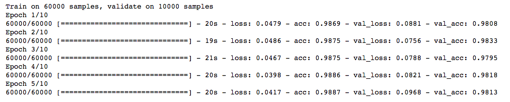
trained_model_5d = model.fit(x_train, y_train, nb_epoch=epochs, batch_size=batch_size, validation_data=(x_test, y_test))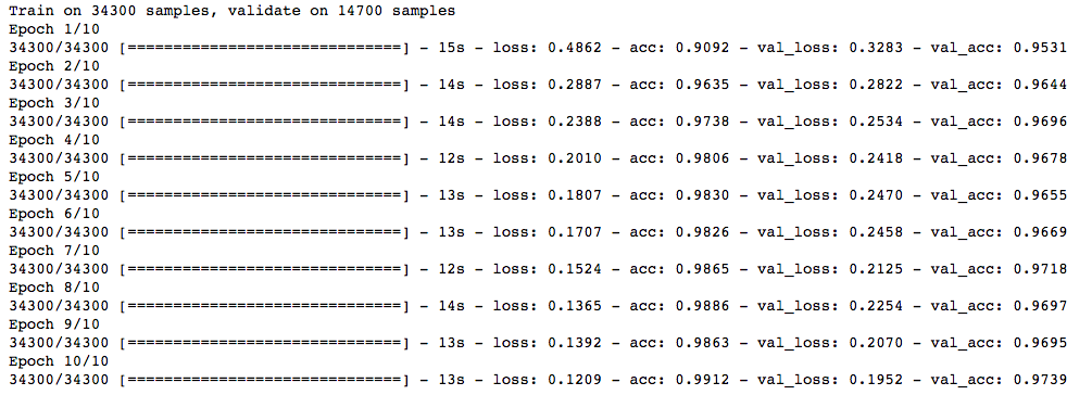
Note that the value of lambda is equal to 0.0001. Great! We just obtained an accuracy which is greater than our previous NN model.
Now, let’s try the L1 regularization technique.
## l1

model = Sequential([
 Dense(output_dim=hidden1_num_units, input_dim=input_num_units, activation='relu',
 kernel_regularizer=regularizers.l1(0.0001)),
 Dense(output_dim=hidden2_num_units, input_dim=hidden1_num_units, activation='relu',
 kernel_regularizer=regularizers.l1(0.0001)),
 Dense(output_dim=hidden3_num_units, input_dim=hidden2_num_units, activation='relu',
 kernel_regularizer=regularizers.l1(0.0001)),
 Dense(output_dim=hidden4_num_units, input_dim=hidden3_num_units, activation='relu',
 kernel_regularizer=regularizers.l1(0.0001)),
 Dense(output_dim=hidden5_num_units, input_dim=hidden4_num_units, activation='relu',
 kernel_regularizer=regularizers.l1(0.0001)),

Dense(output_dim=output_num_units, input_dim=hidden5_num_units, activation='softmax'),
 ])
model.compile(loss='categorical_crossentropy', optimizer='adam', metrics=['accuracy'])
trained_model_5d = model.fit(x_train, y_train, nb_epoch=epochs, batch_size=batch_size, validation_data=(x_test, y_test))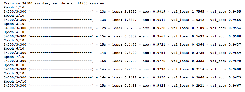
This doesn’t show any improvement over the previous model. Let’s jump to the dropout technique.
## dropout

from keras.layers.core import Dropout
model = Sequential([
 Dense(output_dim=hidden1_num_units, input_dim=input_num_units, activation='relu'),
 Dropout(0.25),
 Dense(output_dim=hidden2_num_units, input_dim=hidden1_num_units, activation='relu'),
 Dropout(0.25),
 Dense(output_dim=hidden3_num_units, input_dim=hidden2_num_units, activation='relu'),
 Dropout(0.25),
 Dense(output_dim=hidden4_num_units, input_dim=hidden3_num_units, activation='relu'),
 Dropout(0.25),
 Dense(output_dim=hidden5_num_units, input_dim=hidden4_num_units, activation='relu'),
 Dropout(0.25),

Dense(output_dim=output_num_units, input_dim=hidden5_num_units, activation='softmax'),
 ])
model.compile(loss='categorical_crossentropy', optimizer='adam', metrics=['accuracy'])
trained_model_5d = model.fit(x_train, y_train, nb_epoch=epochs, batch_size=batch_size, validation_data=(x_test, y_test))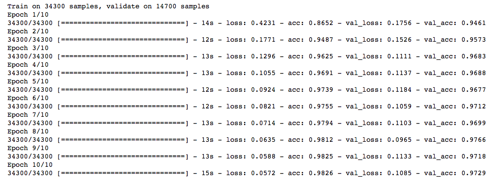
Not bad! Dropout also gives us a little improvement over our simple NN model.
Now, let’s try data augmentation.
from keras.preprocessing.image import ImageDataGenerator
datagen = ImageDataGenerator(zca_whitening=True)

# loading data
train = pd.read_csv(os.path.join(data_dir, 'Train', 'train.csv'))

temp = []
for img_name in train.filename:
 image_path = os.path.join(data_dir, 'Train', 'Images', 'train', img_name)
 img = imread(image_path, flatten=True)
 img = img.astype('float32')
 temp.append(img)

x_train = np.stack(temp)

X_train = x_train.reshape(x_train.shape[0], 1, 28, 28)

X_train = X_train.astype('float32')
Now, fit the training data in order to augment.
# fit parameters from data
datagen.fit(X_train)
Here, I have used zca_whitening as the argument, which highlights the outline of each digit as shown in the image below.
## splitting
y_train = keras.utils.np_utils.to_categorical(train.label.values)
split_size = int(x_train.shape[0]*0.7)

x_train, x_test = X_train[:split_size], X_train[split_size:]
y_train, y_test = y_train[:split_size], y_train[split_size:]
## reshaping
x_train=np.reshape(x_train,(x_train.shape[0],-1))/255
x_test=np.reshape(x_test,(x_test.shape[0],-1))/255## structure using dropout
from keras.layers.core import Dropout
model = Sequential([
Dense(output_dim=hidden1_num_units, input_dim=input_num_units, activation='relu'),
Dropout(0.25),
Dense(output_dim=hidden2_num_units, input_dim=hidden1_num_units, activation='relu'),
Dropout(0.25),
Dense(output_dim=hidden3_num_units, input_dim=hidden2_num_units, activation='relu'),
Dropout(0.25),
Dense(output_dim=hidden4_num_units, input_dim=hidden3_num_units, activation='relu'),
Dropout(0.25),
Dense(output_dim=hidden5_num_units, input_dim=hidden4_num_units, activation='relu'),
Dropout(0.25),
Dense(output_dim=output_num_units, input_dim=hidden5_num_units, activation='softmax'),
])model.compile(loss='categorical_crossentropy', optimizer='adam', metrics=['accuracy'])
trained_model_5d = model.fit(x_train, y_train, nb_epoch=epochs, batch_size=batch_size, validation_data=(x_test, y_test))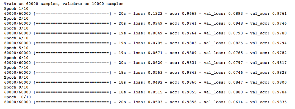
Wow! We got a big leap in the accuracy score. And the good thing is that it works every time. We just need to select a proper argument depending upon the images we have in our dataset.
Now, let’s try our final technique – early stopping.
from keras.callbacks import EarlyStopping
model.compile(loss='categorical_crossentropy', optimizer='adam', metrics=['accuracy'])
trained_model_5d = model.fit(x_train, y_train, nb_epoch=epochs, batch_size=batch_size, validation_data=(x_test, y_test)
 , callbacks = [EarlyStopping(monitor='val_acc', patience=2)])
You can see that our model stops after only 5 iterations as the validation accuracy was not improving. It gives good results in cases where we run it for a larger value of epochs. You can say that it’s a technique to optimize the value of the number of epochs.
Conclusion
I hope that now you have an understanding of regularization in deep learning and the different techniques required to implement it in deep learning models. I highly recommend applying it whenever you are dealing with a deep learning task. It will help you expand your horizons and gain a better understanding of the topic.
Did you find this article helpful? Please share your opinions/thoughts in the comments section below.
Frequently Asked Questions
A. Regularization in deep learning is a technique used to prevent overfitting and improve the generalization of neural networks. It involves adding a regularization term to the loss function, which penalizes large weights or complex model architectures. Regularization methods such as L1 and L2 regularization, dropout, and batch normalization help control model complexity and improve its ability to generalize to unseen data.
A. L1 regularization, also known as Lasso regularization, is a method in deep learning that adds the sum of absolute values of the weights to the loss function. It encourages sparsity by driving some weights to zero, resulting in feature selection. L2 regularization, also called Ridge regularization, adds the sum of squared weights to the loss function, promoting smaller but non-zero weights and preventing extreme values.
A. Dropout is a regularization technique used in neural networks to prevent overfitting. During training, a random subset of neurons is “dropped out” by setting their outputs to zero with a certain probability. This forces the network to learn more robust and independent features, as it cannot rely on specific neurons. Dropout improves generalization and reduces the risk of overfitting.
I am currently pursing my B.Tech in Ceramic Engineering from IIT (B.H.U) Varanasi. I am an aspiring data scientist and a ML enthusiast. I am really passionate about changing the world by using artificial intelligence.


Thanks a lot bro. Immensely helpful.
Could we achieve the same validation accuracy with much lesser architecture ? If so, then our Hyperparameters (especially the L2 lambda) must be quite high (say 0.05). Isn't it ? Or, is there any other way of combating this ??
Thank you for the great article. I'm trying to differentiate between different font weigths of the same font and have been hitting a wall. Was wondering if you could share some insights and if you have had experience with this? What would you recommended as for the best settings, and how big of a dataset would you recommend.