Ever wondered how machines can recognize your face in photos or translate languages in real-time? That’s the magic of neural networks! In this blog, we’ll dive into the different types of neural networks used in deep learning. We’ll break down the popular ones like RNNs, CNNs, ANNs, and LSTMs, RNN VS CNN explaining what makes them special and how they tackle different problems.
So, buckle up and get ready to explore the fascinating world of neural networks!

A neural network is a computational model inspired by the structure and functioning of the human brain. It consists of interconnected nodes, called neurons, organized in layers. Information is processed through these layers, with each neuron receiving inputs, applying a mathematical operation to them, and producing an output. Through a process called training, neural networks can learn to recognize patterns and relationships in data, making them powerful tools for tasks like image and speech recognition, natural language processing, and more.
Here’s a simplified explanation of how it works:
Each neuron in a layer is connected to every neuron in the adjacent layers. The neural network actively adjusts the weights associated with these connections during training to optimize its performance.
As mentioned earlier, each neuron applies an activation function to the weighted sum of its inputs. This function introduces non-linearity into the network, allowing it to learn complex patterns in the data.
Neural networks learn from data through a process called training. During training, the network is fed with input data along with the correct outputs (labels). It adjusts the weights of connections between neurons in order to minimize the difference between its predicted outputs and the true outputs. This process typically involves an optimization algorithm like gradient descent.
Once trained, the neural network can make predictions on new, unseen data by passing it through the network and obtaining the output from the final layer.
In essence, a neural network learns to recognize patterns in data by adjusting its internal parameters (weights) based on examples provided during training, allowing it to generalize and make predictions on new data.
It’s a pertinent question. There is no shortage of machine learning algorithms so why should a data scientist gravitate towards deep learning algorithms? What do neural networks offer that traditional machine learning algorithms don’t?
Another common question I see floating around – neural networks require a ton of computing power, so is it really worth using them? While that question is laced with nuance, here’s the short answer – yes!
The different types of neural networks in deep learning, such as convolutional neural networks (CNN), recurrent neural networks (RNN), artificial neural networks (ANN), etc. are changing the way we interact with the world. These different types of neural networks are at the core of the deep learning revolution, powering applications like unmanned aerial vehicles, self-driving cars, speech recognition, etc.
It’s natural to wonder – can’t machine learning algorithms do the same? Well, here are two key reasons why researchers and experts tend to prefer Deep Learning over Machine Learning:
Curious? Good – let me explain.
Every Machine Learning algorithm learns the mapping from an input to output. In case of parametric models, the algorithm learns a function with a few sets of weights:
Input -> f(w1,w2…..wn) -> OutputIn the case of classification problems, the algorithm learns the function that separates 2 classes – this is known as a Decision boundary. A decision boundary helps us in determining whether a given data point belongs to a positive class or a negative class.
For example, in the case of logistic regression, the learning function is a Sigmoid function that tries to separate the 2 classes:
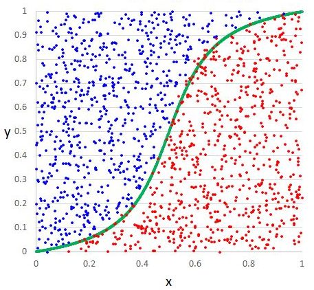
Decision boundary of logistic regression
As you can see here, the logistic regression algorithm learns the linear decision boundary. It cannot learn decision boundaries for nonlinear data like this one:
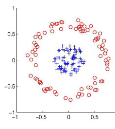
Nonlinear data
Similarly, every Machine Learning algorithm is not capable of learning all the functions. This limits the problems these algorithms can solve that involve a complex relationship.
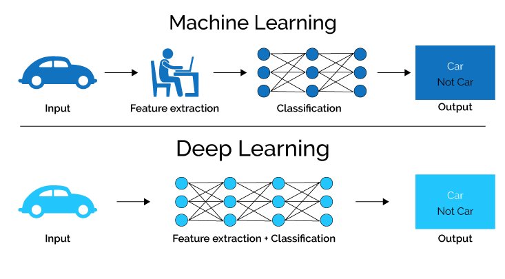
Feature engineering is a key step in the model building process. It is a two-step process:
In feature extraction, we extract all the required features for our problem statement and in feature selection, we select the important features that improve the performance of our machine learning or deep learning model.
Consider an image classification problem. Extracting features manually from an image needs strong knowledge of the subject as well as the domain. It is an extremely time-consuming process. Thanks to Deep Learning, we can automate the process of Feature Engineering!
Now that we understand the importance of deep learning and why it transcends traditional machine learning algorithms, let’s get into the crux of this article. We will discuss the different types of neural networks that you will work with to solve deep learning problems.
If you are just getting started with Machine Learning and Deep Learning, here is a course to assist you in your journey:
This article focuses on three important types of neural networks that form the basis for most pre-trained models in deep learning:
Let’s discuss each neural network in detail.
The perceptron is a fundamental type of neural network used for binary classification tasks. It consists of a single layer of artificial neurons (also known as perceptrons) that take input values, apply weights, and generate an output. The perceptron is typically used for linearly separable data, where it learns to classify inputs into two categories based on a decision boundary. It finds applications in pattern recognition, image classification, and linear regression. However, the perceptron has limitations in handling complex data that is not linearly separable.


LSTM networks are a type of recurrent neural network (RNN) designed to capture long-term dependencies in sequential data. Unlike traditional feedforward networks, LSTM networks have memory cells and gates that allow them to retain or forget information over time selectively. This makes LSTMs effective in speech recognition, natural language processing, time series analysis, and translation. The challenge with LSTM networks lies in selecting the appropriate architecture and parameters and dealing with vanishing or exploding gradients during training.


The RBF neural network is a feedforward neural network that uses radial basis functions as activation functions. RBF networks consist of multiple layers, including an input layer, one or more hidden layers with radial basis activation functions, and an output layer. RBF networks excel in pattern recognition, function approximation, and time series prediction. However, challenges in training RBF networks include selecting appropriate basis functions, determining the number of basis functions, and handling overfitting.


A single perceptron (or neuron) can be imagined as a Logistic Regression. Artificial Neural Network, or ANN, is a group of multiple perceptrons/ neurons at each layer. ANN is also known as a Feed-Forward Neural network because inputs are processed only in the forward direction:

ANN
As you can see here, ANN consists of 3 layers – Input, Hidden and Output. The input layer accepts the inputs, the hidden layer processes the inputs, and the output layer produces the result. Essentially, each layer tries to learn certain weights.
If you want to explore more about how ANN works, I recommend going through the below article:
ANN can be used to solve problems related to:
Artificial Neural Network is capable of learning any nonlinear function. Hence, these networks are popularly known as Universal Function Approximators. ANNs have the capacity to learn weights that map any input to the output.
One of the main reasons behind universal approximation is the activation function. Activation functions introduce nonlinear properties to the network. This helps the network learn any complex relationship between input and output.
Perceptron
As you can see here, the output at each neuron is the activation of a weighted sum of inputs. But wait – what happens if there is no activation function? The network only learns the linear function and can never learn complex relationships. That’s why:
An activation function is a powerhouse of ANN!

ANN: Image classification
In the above scenario, if the size of the image is 224*224, then the number of trainable parameters at the first hidden layer with just 4 neurons is 602,112. That’s huge!

Backward Propagation
So, in the case of a very deep neural network (network with a large number of hidden layers), the gradient vanishes or explodes as it propagates backward which leads to vanishing and exploding gradient.
Now, let us see how to overcome the limitations of MLP using two different architectures – Recurrent Neural Networks (RNN) and Convolution Neural Networks (CNN).
Let us first try to understand the difference between an RNN and an ANN from the architecture perspective:
A looping constraint on the hidden layer of ANN turns to RNN.
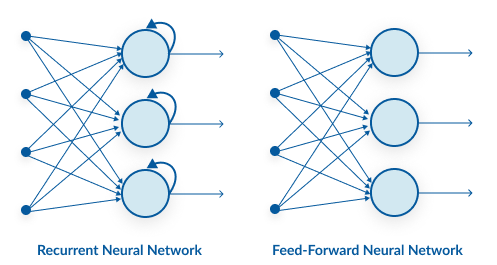
As you can see here, RNN has a recurrent connection on the hidden state. This looping constraint ensures that sequential information is captured in the input data.
You should go through the below tutorial to learn more about how RNNs work under the hood (and how to build one in Python):
We can use recurrent neural networks to solve the problems related to:
Many2Many Seq2Seq model
As you can see here, the output (o1, o2, o3, o4) at each time step depends not only on the current word but also on the previous words.

Unrolled RNN
As shown in the above figure, 3 weight matrices – U, W, V, are the weight matrices that are shared across all the time steps.
Deep RNNs (RNNs with a large number of time steps) also suffer from the vanishing and exploding gradient problem which is a common problem in all the different types of neural networks.

Vanishing Gradient (RNN)
As you can see here, the gradient computed at the last time step vanishes as it reaches the initial time step.
Convolutional neural networks (CNN) are all the rage in the deep learning community right now. These CNN models are being used across different applications and domains, and they’re especially prevalent in image and video processing projects.
The building blocks of CNNs are filters a.k.a. kernels. Kernels are used to extract the relevant features from the input using the convolution operation. Let’s try to grasp the importance of filters using images as input data. Convolving an image with filters results in a feature map:

Output of Convolution
Want to explore more about Convolution Neural Networks? I recommend going through the below tutorial:
You can also enrol in this free course on CNN to learn more about them: Convolutional Neural Networks from Scratch
Though convolutional neural networks were introduced to solve problems related to image data, they perform impressively on sequential inputs as well.
CNN – Image Classification

In the above image, we can easily identify that its a human’s face by looking at specific features like eyes, nose, mouth and so on. We can also see how these specific features are arranged in an image. That’s exactly what CNNs are capable of capturing.
Convolving image with a filter
Notice that the 2*2 feature map is produced by sliding the same 3*3 filter across different parts of an image.
Here, I have summarized some of the differences among different types of neural networks:

In this article, I have discussed the importance of deep learning and the differences among different types of neural networks. I strongly believe that knowledge sharing is the ultimate form of learning. I am looking forward to hearing a few more differences!
Hope you like the article and get to know about the types of neural networks and how its performing and what impact it’s creating.
A. The three different types of neural networks are:
1. Feedforward Neural Networks (FFNN)
2. Recurrent Neural Networks (RNN)
3. Convolutional Neural Networks (CNN).
A. RNN stands for Recurrent Neural Network, a type of neural network designed to process sequential data by retaining memory of past inputs through hidden states. Convolutional Neural Networks, also known as CNNs, leverage convolution operations for image recognition and processing tasks.
A. The two neural networks referred to commonly are:
1. Artificial Neural Networks (ANN)
2. Convolutional Neural Networks (CNN)
A. The best type of neural network depends on your problem. Convolutional Neural Networks rule image recognition, Long Short-Term Memory networks tackle sequential data like speech, and Recurrent Neural Networks are their foundational cousin. Tell me more about your specific task, and I can recommend a powerful neural network architecture to conquer it.
Lorem ipsum dolor sit amet, consectetur adipiscing elit,


good one. Refreshing the concepts in quick time . :) :) Thanks !
A great Brief on types of NNs precisely done. Splendid. I wish it were an ebook. Thanks
That is a good one Aravind. Helpful. Thanks
Wow, great visualization! Thank you!
Excellent visual explanation. Just had to know CNN/RNN quickly in data analytics for fraud calls detection. Nice job and Rahul Dravid made me even more happier! Thank you
This is good one very knowledge
it's very good. Thank you very much. very useful and nice.
Very nice and informative. Thanks!
Thank you very much! You concisely wrapped up the whole concepts, nice quick refresher!
Thank you so much for the Very Valuable Article
Thank you, great stuff.
Thanks guys for clearing the air for me (Similarities and differences among ANN, RNN and CNN)
Nice Explanation. Easy to understand. Please provide more tutorials like this in the fields of your interest.
Self explanatory. It was Excellent
Great article! I found the explanations of the different types of neural networks in deep learning to be very helpful. As a beginner in this field, it's not always easy to understand the differences between different architectures, but this post did a great job of breaking it down in a clear and concise manner. Thanks for sharing your knowledge!