Introduction
In my previous article, I discussed the implementation of neural networks using TensorFlow. Continuing the series of articles on neural network libraries, I have decided to throw light on Keras – supposedly the best deep learning library so far.
I have been working on deep learning for sometime now and according to me, the most difficult thing when dealing with Neural Networks is the never-ending range of parameters to tune. With increase in depth of a Neural Network, it becomes increasingly difficult to take care of all the parameters. Mostly, people rely on intuition and experience to tune it. In reality, research is still rampant on this topic.

Thankfully we have Keras, which takes care of a lot of this hard work and provides an easier interface!
In this article, I am going to share my experience of working in deep learning. We will begin with an overview of Keras, its features and differentiation over other libraries. We will then, look at a simple implementation of neural networks in Keras. And then, I will take you through a hands-on exercise on parameter tuning in neural networks.
Table of Contents
-
- Keras : Overview
- Keras: Advantages
- Keras: Limitations
- General way to solve problems with Neural Networks
- Starting with a simple Keras implementation on “Identify the Digits”
- Hyperparameters to look out for in Neural Networks
- Getting your hands dirty (Parameter Tuning)
- Where to go from here?
- Additional Resources
1. Keras : Overview
![]()
Keras is a high level library, used specially for building neural network models. It is written in Python and is compatible with both Python – 2.7 & 3.5. Keras was specifically developed for fast execution of ideas. It has a simple and highly modular interface, which makes it easier to create even complex neural network models. This library abstracts low level libraries, namely Theano and TensorFlow so that, the user is free from “implementation details” of these libraries.
The key features of Keras are:
- Modularity : Modules necessary for building a neural network are included in a simple interface so that Keras is easier to use for the end user.
- Minimalistic : Implementation is short and concise.
- Extensibility : It’s very easy to write a new module for Keras and makes it suitable for advance research.
2. Keras : Advantages
Being a high level library and its simpler interface, Keras certainly shines as one of the best deep learning library available. Few features of Keras, which stands out in comparison with other libraries are:
- In comparison to Theano and TensorFlow, it takes in all the advantages of both of these libraries and tries to give a better “user experience”.
- As Keras is a python library, it is more accessible to general public because of Python’s inherent simplicity as a programming language.
- A similar library in comparison to Keras is Lasagne, but having used both I can say that Keras is much easier to use.
Given the above reasons, it is no surprise that Keras is increasingly becoming popular as a deep learning library.
3. Keras : Limitations
- I think that having a dependency on low level libraries like Theano / TensorFlow is a double edged sword. This is because Keras cannot go “out of the realms” of these libraries. For example, both Theano and TensorFlow do not support GPUs other than Nvidia (currently). And hence, Keras too doesn’t have the corresponding support.
- Also unlike Lasagne, Keras completely abstracts the low level languages. So, it is less flexible when it comes to building custom operations.
- The last point I’ll make is that Keras is relatively new. The first version was released in early 2015, and it has undergone many changes since then. Although Keras is already used in production, but you should think twice before deploying keras models for productions.
4. General way to solve problems with Neural Networks
Neural networks is a special type of machine learning (ML) algorithm. So, like every ML algorithm, it follows the usual ML workflow of data preprocessing, model building and model evaluation. For the sake of conciseness, I have listed out a To-D0 list of how to approach a Neural Network problem.
- Check if it is a problem where Neural Network gives you uplift over traditional algorithms (refer to the checklist in the section above)
- Do a survey of which Neural Network architecture is most suitable for the required problem
- Define Neural Network architecture through whichever language / library you choose.
- Convert data to right format and divide it in batches
- Pre-process the data according to your needs
- Augment Data to increase size and make better trained models
- Feed batches to Neural Network
- Train and monitor changes in training and validation data sets
- Test your model, and save it for future use
5. Starting with a simple Keras implementation on “Identify the Digits”
Before starting this experiment, make sure you have Keras installed in your system. Refer the official installation guide. We will use tensorflow for backend, so make sure you have this done in your config file. If not, follow the steps given here.
Here, we solve our deep learning practice problem – Identify the Digits. Let’s take a look at our problem statement:
Our problem is an image recognition problem, to identify digits from a given 28 x 28 image. We have a subset of images for training and the rest for testing our model. So first, download the train and test files. The dataset contains a zipped file of all the images and both the train.csv and test.csv have the name of corresponding train and test images. Any additional features are not provided in the datasets, just the raw images are provided in ‘.png’ format.
Let’s start:
STEP 0: Getting Ready
a) Import all the necessary libraries
%pylab inline
import os
import numpy as np
import pandas as pd
from scipy.misc import imread
from sklearn.metrics import accuracy_score

import tensorflow as tf
import keras
b) Let’s set a seed value, so that we can control our models randomness
# To stop potential randomness
seed = 128
rng = np.random.RandomState(seed)
c) The first step is to set directory paths, for safekeeping!
root_dir = os.path.abspath('../..')data_dir = os.path.join(root_dir, 'data')sub_dir = os.path.join(root_dir, 'sub')# check for existenceos.path.exists(root_dir)os.path.exists(data_dir)os.path.exists(sub_dir)
STEP 1: Data Loading and Preprocessing
a) Now let us read our datasets. These are in .csv formats, and have a filename along with the appropriate labels
train = pd.read_csv(os.path.join(data_dir, 'Train', 'train.csv'))
test = pd.read_csv(os.path.join(data_dir, 'Test.csv'))

sample_submission = pd.read_csv(os.path.join(data_dir, 'Sample_Submission.csv'))

train.head()
| filename | label | |
|---|---|---|
| 0 | 0.png | 4 |
| 1 | 1.png | 9 |
| 2 | 2.png | 1 |
| 3 | 3.png | 7 |
| 4 | 4.png | 3 |
b) Let us see what our data looks like! We read our image and display it.
img_name = rng.choice(train.filename)
filepath = os.path.join(data_dir, 'Train', 'Images', 'train', img_name)

img = imread(filepath, flatten=True)

pylab.imshow(img, cmap='gray')
pylab.axis('off')
pylab.show()
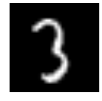
c) The above image is represented as numpy array, as seen below
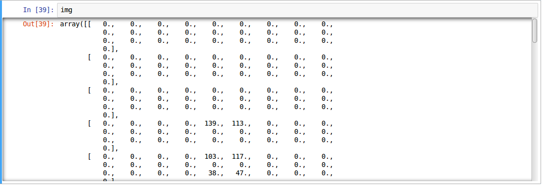
d) For easier data manipulation, let’s store all our images as numpy arrays
temp = []
for img_name in train.filename:
    image_path = os.path.join(data_dir, 'Train', 'Images', 'train', img_name)
    img = imread(image_path, flatten=True)
    img = img.astype('float32')
    temp.append(img)

train_x = np.stack(temp)

train_x /= 255.0
train_x = train_x.reshape(-1, 784).astype('float32')

temp = []
for img_name in test.filename:
    image_path = os.path.join(data_dir, 'Train', 'Images', 'test', img_name)
    img = imread(image_path, flatten=True)
    img = img.astype('float32')
    temp.append(img)

test_x = np.stack(temp)

test_x /= 255.0
test_x = test_x.reshape(-1, 784).astype('float32')
train_y = keras.utils.np_utils.to_categorical(train.label.values)
e) As this is a typical ML problem, to test the proper functioning of our model we create a validation set. Let’s take a split size of 70:30 for train set vs validation set
split_size = int(train_x.shape[0]*0.7)

train_x, val_x = train_x[:split_size], train_x[split_size:]
train_y, val_y = train_y[:split_size], train_y[split_size:]
train.label.ix[split_size:]
STEP 2: Model Building
a) Now comes the main part! Let us define our neural network architecture. We define a neural network with 3 layers input, hidden and output. The number of neurons in input and output are fixed, as the input is our 28 x 28 image and the output is a 10 x 1 vector representing the class. We take 50 neurons in the hidden layer. Here, we use Adam as our optimization algorithms, which is an efficient variant of Gradient Descent algorithm. There are a number of other optimizers available in keras (refer here). In case you don’t understand any of these terminologies, check out the article on fundamentals of neural network to know more in depth of how it works.
# define vars
input_num_units = 784
hidden_num_units = 50
output_num_units = 10

epochs = 5
batch_size = 128

# import keras modules

from keras.models import Sequential
from keras.layers import Dense

# create model
model = Sequential([
  Dense(output_dim=hidden_num_units, input_dim=input_num_units, activation='relu'),
  Dense(output_dim=output_num_units, input_dim=hidden_num_units, activation='softmax'),
])

# compile the model with necessary attributes
model.compile(loss='categorical_crossentropy', optimizer='adam', metrics=['accuracy'])
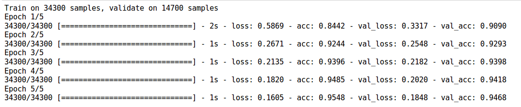
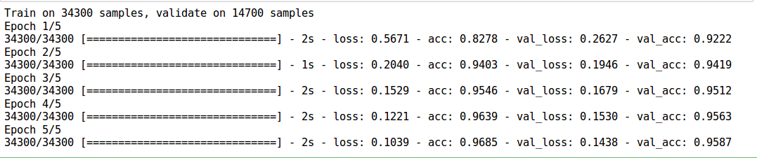
b) It’s time to train our model
trained_model = model.fit(train_x, train_y, nb_epoch=epochs, batch_size=batch_size, validation_data=(val_x, val_y))
STEP 3: Model Evaluation
a) To test our model with our own eyes, let’s visualize its predictions
pred = model.predict_classes(test_x)

img_name = rng.choice(test.filename)
filepath = os.path.join(data_dir, 'Train', 'Images', 'test', img_name)

img = imread(filepath, flatten=True)

test_index = int(img_name.split('.')[0]) - train.shape[0]

print "Prediction is: ", pred[test_index]

pylab.imshow(img, cmap='gray')
pylab.axis('off')
pylab.show()

Prediction is:  8

b) We see that our model performs well even on being very simple. Now we create a submission with our model
sample_submission.filename = test.filename; sample_submission.label = pred
sample_submission.to_csv(os.path.join(sub_dir, 'sub02.csv'), index=False)
6. Hyperparameters to look out for in Neural Networks
 I feel that, hyperparameter tuning is the hardest in neural network in comparison to any other machine learning algorithm. You would be insane to apply Grid Search, as there are numerous parameters when it comes to tuning a neural network.
Note: I have discussed a few more details, on when to apply neural networks in the following article An Introduction to Implementing Neural Networks using TensorFlow
Some important parameters to look out for while optimizing neural networks are:
- Type of architecture
- Number of Layers
- Number of Neurons in a layer
- Regularization parameters
- Learning Rate
- Type of optimization / backpropagation technique to use
- Dropout rate
- Weight sharing
Also, there may be many more hyperparameters depending on the type of architecture. For example, if you use a convolutional neural network, you would have to look at hyperparameters like convolutional filter size, pooling value, etc.
The best way to pick good parameters is to understand your problem domain. Research the previously applied techniques on your data, and most importantly ask experienced people for insights to the problem. It’s the only way you can try to ensure you get a “good enough” neural network model.
Here are some resources for tips and tricks for training neural networks. (Resource 1, Resource 2, Resource 3)
7. Getting your hands dirty
Let us take our knowledge of hyperparameters and start tweaking our neural network model.
- As we did before, we redo all the pre-requisite things. Let’s import the modules
%pylab inline

import os
import numpy as np
import pandas as pd
from scipy.misc import imread
from sklearn.metrics import accuracy_score
import tensorflow as tf
import keras

from keras.models import Sequential
from keras.layers import Dense, Activation, Dropout, Convolution2D, Flatten, MaxPooling2D, Reshape, InputLayer
- As before, set seed value
# To stop potential randomness
seed = 128
rng = np.random.RandomState(seed)
- Set paths for further use
root_dir = os.path.abspath('../..')
data_dir = os.path.join(root_dir, 'data')
sub_dir = os.path.join(root_dir, 'sub')

# check for existence
os.path.exists(root_dir)
os.path.exists(data_dir)
os.path.exists(sub_dir)
- Read the datasets and convert them to usable form
train = pd.read_csv(os.path.join(data_dir, 'Train', 'train.csv'))
test = pd.read_csv(os.path.join(data_dir, 'Test.csv'))

sample_submission = pd.read_csv(os.path.join(data_dir, 'Sample_Submission.csv'))

temp = []
for img_name in train.filename:
  image_path = os.path.join(data_dir, 'Train', 'Images', 'train', img_name)
  img = imread(image_path, flatten=True)
  img = img.astype('float32')
  temp.append(img)

train_x = np.stack(temp)

train_x /= 255.0
train_x = train_x.reshape(-1, 784).astype('float32')

temp = []
for img_name in test.filename:
  image_path = os.path.join(data_dir, 'Train', 'Images', 'test', img_name)
  img = imread(image_path, flatten=True)
  img = img.astype('float32')
  temp.append(img)

test_x = np.stack(temp)

test_x /= 255.0
test_x = test_x.reshape(-1, 784).astype('float32')

train_y = keras.utils.np_utils.to_categorical(train.label.values)
- Divide our train data into training and validation
split_size = int(train_x.shape[0]*0.7)

train_x, val_x = train_x[:split_size], train_x[split_size:]
train_y, val_y = train_y[:split_size], train_y[split_size:]
- Let’s start our tweaking! Lets change our model to be “wide”, i.e. increase the number of neurons in our hidden layer
# define vars
input_num_units = 784
hidden_num_units = 500
output_num_units = 10
epochs = 5
batch_size = 128

model = Sequential([
 Dense(output_dim=hidden_num_units, input_dim=input_num_units, activation='relu'),

 Dense(output_dim=output_num_units, input_dim=hidden_num_units, activation='softmax'),
])
- Let’s test this model
model.compile(loss='categorical_crossentropy', optimizer='adam', metrics=['accuracy'])

trained_model_500 = model.fit(train_x, train_y, nb_epoch=epochs, batch_size=batch_size, validation_data=(val_x, val_y))
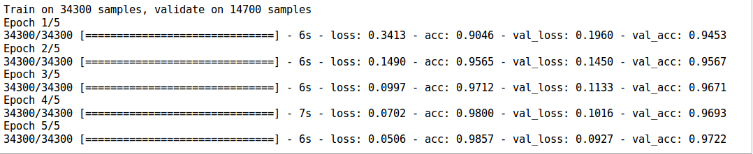
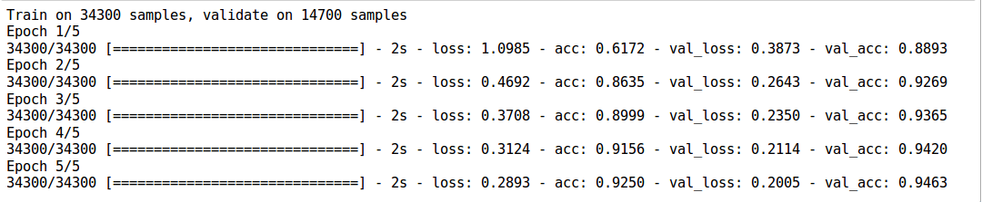
- We see that this model performs significantly better than before! Now instead of “wide”, we try making our model “deep”. We add four more hidden layers with 50 neurons each
# define vars
input_num_units = 784
hidden1_num_units = 50
hidden2_num_units = 50
hidden3_num_units = 50
hidden4_num_units = 50
hidden5_num_units = 50
output_num_units = 10

epochs = 5
batch_size = 128

model = Sequential([
 Dense(output_dim=hidden1_num_units, input_dim=input_num_units, activation='relu'),
 Dense(output_dim=hidden2_num_units, input_dim=hidden1_num_units, activation='relu'),
 Dense(output_dim=hidden3_num_units, input_dim=hidden2_num_units, activation='relu'),
 Dense(output_dim=hidden4_num_units, input_dim=hidden3_num_units, activation='relu'),
 Dense(output_dim=hidden5_num_units, input_dim=hidden4_num_units, activation='relu'),

Dense(output_dim=output_num_units, input_dim=hidden5_num_units, activation='softmax'),
 ])
- Any guesses on how this model would perform?
model.compile(loss='categorical_crossentropy', optimizer='adam', metrics=['accuracy'])

trained_model_5d = model.fit(train_x, train_y, nb_epoch=epochs, batch_size=batch_size, validation_data=(val_x, val_y))
- Looks like we didn’t get what we expected. This may be because our model may be overfitting. To deal with this, we use a method called dropout. Dropout is essentially randomly turning off parts of the model so that it does not “overlearn” a concept (To read more about dropout, check out the article on core concepts of neural networks)
# define vars
input_num_units = 784
hidden1_num_units = 50
hidden2_num_units = 50
hidden3_num_units = 50
hidden4_num_units = 50
hidden5_num_units = 50
output_num_units = 10

epochs = 5
batch_size = 128

dropout_ratio = 0.2

model = Sequential([
 Dense(output_dim=hidden1_num_units, input_dim=input_num_units, activation='relu'),
 Dropout(dropout_ratio),
 Dense(output_dim=hidden2_num_units, input_dim=hidden1_num_units, activation='relu'),
 Dropout(dropout_ratio),
 Dense(output_dim=hidden3_num_units, input_dim=hidden2_num_units, activation='relu'),
 Dropout(dropout_ratio),
 Dense(output_dim=hidden4_num_units, input_dim=hidden3_num_units, activation='relu'),
 Dropout(dropout_ratio),
 Dense(output_dim=hidden5_num_units, input_dim=hidden4_num_units, activation='relu'),
 Dropout(dropout_ratio),

Dense(output_dim=output_num_units, input_dim=hidden5_num_units, activation='softmax'),
 ])
- Now let’s check our accuracy
model.compile(loss='categorical_crossentropy', optimizer='adam', metrics=['accuracy'])

trained_model_5d_with_drop = model.fit(train_x, train_y, nb_epoch=epochs, batch_size=batch_size, validation_data=(val_x, val_y))
- Something seems off. It seems that our model is not performing well enough. One reason may be because we are not training our model to its full potential. Increase our training epochs to 50 and check it out!
# define vars
input_num_units = 784
hidden1_num_units = 50
hidden2_num_units = 50
hidden3_num_units = 50
hidden4_num_units = 50
hidden5_num_units = 50
output_num_units = 10

epochs = 50
batch_size = 128
model = Sequential([
 Dense(output_dim=hidden1_num_units, input_dim=input_num_units, activation='relu'),
 Dropout(0.2),
 Dense(output_dim=hidden2_num_units, input_dim=hidden1_num_units, activation='relu'),
 Dropout(0.2),
 Dense(output_dim=hidden3_num_units, input_dim=hidden2_num_units, activation='relu'),
 Dropout(0.2),
 Dense(output_dim=hidden4_num_units, input_dim=hidden3_num_units, activation='relu'),
 Dropout(0.2),
 Dense(output_dim=hidden5_num_units, input_dim=hidden4_num_units, activation='relu'),
 Dropout(0.2),

Dense(output_dim=output_num_units, input_dim=hidden5_num_units, activation='softmax'),
])
- Well I’m excited to see what will happen. Are you?
model.compile(loss='categorical_crossentropy', optimizer='adam', metrics=['accuracy'])

trained_model_5d_with_drop_more_epochs = model.fit(train_x, train_y, nb_epoch=epochs, batch_size=batch_size, validation_data=(val_x, val_y))
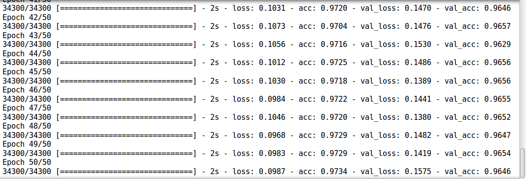
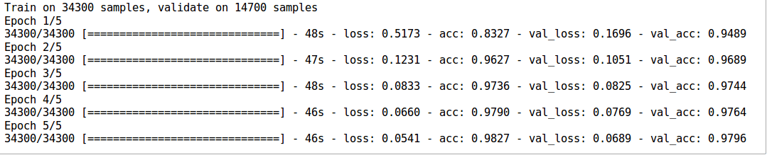
- Yes! this is good. We see an increase in accuracy. (As an optional assignment, you could try increasing number of epochs to train more) Let’s try another thing, we make our model both deep and wide! We also implement all the tweaks that we learnt before. For the purpose of getting faster results, we reduce the training epochs. But you are free to increase them if you want.
# define vars
input_num_units = 784
hidden1_num_units = 500
hidden2_num_units = 500
hidden3_num_units = 500
hidden4_num_units = 500
hidden5_num_units = 500
output_num_units = 10

epochs = 25
batch_size = 128

model = Sequential([
 Dense(output_dim=hidden1_num_units, input_dim=input_num_units, activation='relu'),
 Dropout(0.2),
 Dense(output_dim=hidden2_num_units, input_dim=hidden1_num_units, activation='relu'),
 Dropout(0.2),
 Dense(output_dim=hidden3_num_units, input_dim=hidden2_num_units, activation='relu'),
 Dropout(0.2),
 Dense(output_dim=hidden4_num_units, input_dim=hidden3_num_units, activation='relu'),
 Dropout(0.2),
 Dense(output_dim=hidden5_num_units, input_dim=hidden4_num_units, activation='relu'),
 Dropout(0.2),

Dense(output_dim=output_num_units, input_dim=hidden5_num_units, activation='softmax'),
 ])
- Forgive me for the spoliers, but its clear that our model would be better than all our models before.
 Still lets check it out
model.compile(loss='categorical_crossentropy', optimizer='adam', metrics=['accuracy'])

trained_model_deep_n_wide = model.fit(train_x, train_y, nb_epoch=epochs, batch_size=batch_size, validation_data=(val_x, val_y))
- Seems like we broke all the records! Lets submit this model to the solution checker
pred = model.predict_classes(test_x)
 sample_submission.filename = test.filename; sample_submission.label = pred
 sample_submission.to_csv(os.path.join(sub_dir, 'sub03.csv'), index=False)
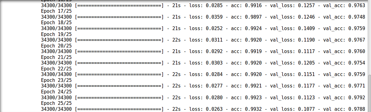
- As a last tweak, we will try changing the type of our model. Until now we made multilayer perceptrons (MLP). Let’s now change it to a convolutional neural network. (To get an in-depth introduction to convolutional neural network (CNN), go through this article). One thing necessary for running a CNN is that it requires to be arranged in a specific format. So let’s reshape our data and feed it to our CNN.
# reshape data

train_x_temp = train_x.reshape(-1, 28, 28, 1)
val_x_temp = val_x.reshape(-1, 28, 28, 1)

# define vars
input_shape = (784,)
input_reshape = (28, 28, 1)

conv_num_filters = 5
conv_filter_size = 5

pool_size = (2, 2)

hidden_num_units = 50
output_num_units = 10

epochs = 5
batch_size = 128

model = Sequential([
 InputLayer(input_shape=input_reshape),

 Convolution2D(25, 5, 5, activation='relu'),
 MaxPooling2D(pool_size=pool_size),

 Convolution2D(25, 5, 5, activation='relu'),
 MaxPooling2D(pool_size=pool_size),

 Convolution2D(25, 4, 4, activation='relu'),

 Flatten(),

 Dense(output_dim=hidden_num_units, activation='relu'),

 Dense(output_dim=output_num_units, input_dim=hidden_num_units, activation='softmax'),
])

model.compile(loss='categorical_crossentropy', optimizer='adam', metrics=['accuracy'])

trained_model_conv = model.fit(train_x_temp, train_y, nb_epoch=epochs, batch_size=batch_size, validation_data=(val_x_temp, val_y))
This result blows your mind, doesn’t it. Even with such small training time, the performance is way better! This proves that a better architecture can certainly boost your performance when dealing with neural networks.
It’s time to let go of the training wheels. There’s many things you can try, so many tweaks to do. Try this on your end and let us know how it goes!
8. Where to go from here?
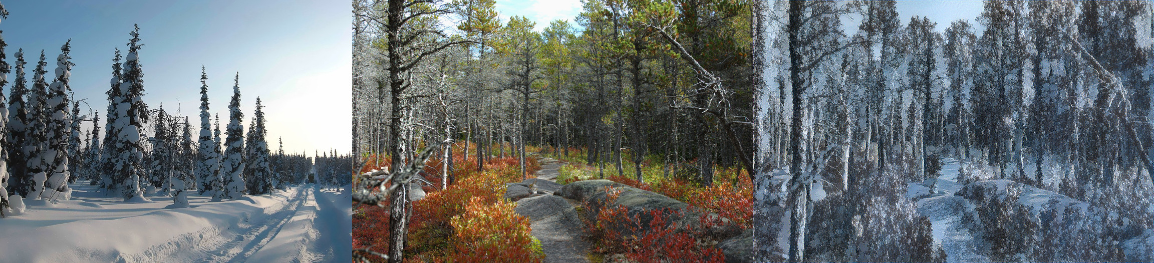
Now, you have a basic overview of Keras and a hands-on experience of implementing neural networks. There is still much more you can do. For example, I really like the implementation of keras to build image analogies. In this project, the authors train a neural network to understand an image, and recreate learnt attributes to another image. As seen below, the first two images are given as input, where the model trains on the first image and on giving input as second image, gives output as the third image.
Neural network tuning is still considered as a “dark art”. So, don’t expect that you would get the best model in your first try. Build, evaluate and reiterate, this is how you would be a better neural network practitioner.
Another point you should know that there are other methods to ensure that you would get a “good enough” neural network model without training it from scratch. Techniques like pre-training and transfer learning, are essential to know when you are implementing neural network models to solve real life problems.
9. Additional Resources
End Notes
I hope you found this article helpful. Now, it’s time for you to practice and read as much as you can. Good luck! If you have any recommendations / suggestions on neural networks, I’d love to interact with you in comments. If you have any more doubts or queries feel to drop in your comments below. Try out the practice problem Identify the Digits yourself and let me know what was your experience.
Faizan is a Data Science enthusiast and a Deep learning rookie. A recent Comp. Sc. undergrad, he aims to utilize his skills to push the boundaries of AI research.


Very useful for the people who is looking for NN with Python. Keras is the power ful package for NN when compared to other packages available
Thanks! Hope it helps others too
Hi Great Article thank you . One clarification I am unable to install tensorflow in windows is it only for mac? Thanks
Hello Pradeep. Unfortunately windows is still not supported now (october 2016: refer this issue https://github.com/tensorflow/tensorflow/issues/17). On the other hand, you could try installing linux on virtual machine or in a docker container. (for docker refer here http://www.netinstructions.com/how-to-install-and-run-tensorflow-on-a-windows-pc/)
Hello Faizan, I have been following your posts on deep learning, they are simple and easy to follow. Could you please help me with the hardware (cost effective for students) requirement for deep learning, so that it can run data sets listed here https://github.com/ChristosChristofidis/awesome-deep-learning.
Hello Venkat. Its great that your following the articles. Do hold on as there are may more of these to come! To answer your question; small or medium datasets are runnable on a typical laptop given enough time. I personally have an HP-Pavilion laptop with i5 processor, 4GB RAM and 2GB Nvidia GT740M. For bigger datasets like ImageNet which have hundreds of GBs I would suggest you move on to bigger machines. As you are still a student, you could request your college for a machine with good specs. For my BE project, I used my college's workstation (i7, 8GB RAM, 12 GB Nvidia Titan X) I wrote a note on how to setup your machine for deep learning, do go through it (step 1 of this article https://www.analyticsvidhya.com/blog/2016/08/deep-learning-path/)