Multivariate Time Series Analysis With Python for Forecasting and Modeling (Updated 2023)

Introduction

Time is the most critical factor in data science and machine learning that decides whether a business will rise or fall. That’s why we see sales in stores and e-commerce platforms aligning with festivals. These businesses analyze years of spending data to understand the best time to throw open the gates and see an increase in consumer spending.

But how can you, as a data scientist, perform this analysis? Don’t worry, you don’t need to build a time machine! Time Series modeling is a powerful technique that acts as a gateway to understanding and forecasting trends and patterns.

But even a time series model has different facets. Most of the examples we see on the web deal with univariate time series. Unfortunately, real-world use cases don’t work like that. There are multiple variables at play, and handling all of them at the same time is where a data scientist will earn his worth.

Learning Objectives

• Understand what a multivariate time series is and how to deal with it.
• Understand the difference between univariate and multivariate time series.
• Learn the implementation of multivariate time series in Python following a case study-based tutorial.

Univariate Vs. Multivariate Time Series Forecasting Python

This article assumes some familiarity with univariate time series, their properties, and various techniques used for forecasting. Since this article will be focused on multivariate time series, I would suggest you go through the following articles, which serve as a good introduction to univariate time series:

• Comprehensive guide to creating time series forecast
• Build high-performance time series models using Auto Arima

But I’ll give you a quick refresher on what a univariate time series is before going into the details of a multivariate time series. Let’s look at them one by one to understand the difference.

Univariate Time Series

A univariate time series, as the name suggests, is a series with a single time-dependent variable.

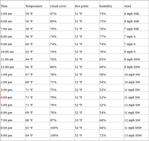
For example, have a look at the sample dataset below, which consists of the temperature values (each hour) for the past 2 years. Here, the temperature is the dependent variable (dependent on Time).

If we are asked to predict the temperature for the next few days, we will look at the past values and try to gauge and extract a pattern. We would notice that the temperature is lower in the morning and at night while peaking in the afternoon. Also, if you have data for the past few years, you would observe that it is colder during the months of November to January while being comparatively hotter from April to June.

Such observations will help us in predicting future values. Did you notice that we used only one variable (the temperature of the past 2 years)? Therefore, this is called Univariate Time Series Analysis/Forecasting.

Multivariate Time Series (MTS)

A Multivariate time series has more than one time series variable. Each variable depends not only on its past values but also has some dependency on other variables. This dependency is used for forecasting future values. Sounds complicated? Let me explain.

Consider the above example. Suppose our dataset includes perspiration percent, dew point, wind speed, cloud cover percentage, etc., and the temperature value for the past two years. In this case, multiple variables must be considered to predict temperature optimally. A series like this would fall under the category of multivariate time series. Below is an illustration of this:

Now that we understand what a multivariate time series looks like, let us understand how we can use it to build a forecast.

Dealing With a Multivariate Time Series – VAR

In this section, I will introduce you to one of the most commonly used methods for multivariate time series forecasting – Vector Auto Regression (VAR).

In a VAR algorithm, each variable is a linear function of the past values of itself and the past values of all the other variables. To explain this in a better manner, I’m going to use a simple visual example:

We have two variables, y1, and y2. We need to forecast the value of these two variables at a time ‘t’ from the given data for past n values. For simplicity, I have considered the lag value to be 1.

To compute y1(t), we will use the past value of y1 and y2. Similarly, to compute y2(t), past values of both y1 and y2 will be used. Below is a simple mathematical way of representing this relation:

Here,

• a1 and a2 are the constant terms,
• w11, w12, w21, and w22 are the coefficients,
• e1 and e2 are the error terms

These equations are similar to the equation of an AR process. Since the AR process is used for univariate time series data, the future values are linear combinations of their own past values only. Consider the AR(1) process:

y(t) = a + w*y(t-1) +e

In this case, we have only one variable – y, a constant term – a, an error term – e, and a coefficient – w. In order to accommodate the multiple variable terms in each equation for VAR, we will use vectors.  We can write equations (1) and (2) in the following form:

The two variables are y1 and y2, followed by a constant, a coefficient metric, a lag value, and an error metric. This is the vector equation for a VAR(1) process. For a VAR(2) process, another vector term for time (t-2) will be added to the equation to generalize for p lags:

The above equation represents a VAR(p) process with variables y1, y2 …yk. The same can be written as:

The term ε_t in the equation represents multivariate vector white noise. For a multivariate time series, ε_t should be a continuous random vector that satisfies the following conditions:

1. E(ε_t) = 0
   The expected value for the error vector is 0
2. E(ε_t1,ε_t2‘) = σ₁₂
   The expected value of ε_t and ε_t‘ is the standard deviation of the series.

Why Do We Need Vector Autoregressive Models?

Recall the temperate forecasting example we saw earlier. An argument can be made for it to be treated as a multiple univariate series. We can solve it using simple univariate forecasting methods like AR. Since the aim is to predict the temperature, we can simply remove the other variables (except temperature) and fit a model on the remaining univariate series.

Another simple idea is to forecast values for each series individually using the techniques we already know. This would make the work extremely straightforward! Then why should you learn another forecasting technique? Isn’t this topic complicated enough already?

From the above equations (1) and (2), it is clear that each variable is using the past values of every variable to make predictions. Unlike AR, VAR is able to understand and use the relationship between several variables. This is useful for describing the dynamic behavior of the data and also provides better forecasting results. Additionally, implementing VAR is as simple as using any other univariate technique (which you will see in the last section).

The extensive usage of VAR models in finance, econometrics, and macroeconomics can be attributed to their ability to provide a framework for achieving significant modeling objectives. With VAR models, it is possible to elucidate the values of endogenous variables by considering their previously observed values.

Granger’s Causality Test

Granger’s causality test can be used to identify the relationship between variables prior to model building. This is important because if there is no relationship between variables, they can be excluded and modeled separately. Conversely, if a relationship exists, the variables must be considered in the modeling phase.

The test in mathematics yields a p-value for the variables. If the p-value exceeds 0.05, the null hypothesis must be accepted. Conversely, if the p-value is less than 0.05, the null hypothesis must be rejected.

Stationarity of a Multivariate Time Series

We know from studying the univariate concept that a stationary time series will, more often than not, give us a better set of predictions. If you are not familiar with the concept of stationarity, please go through this article first: A Gentle Introduction to handling non-stationary Time Series.

To summarize, for a given univariate time series:

y(t) = c*y(t-1) + ε t

The series is said to be stationary if the value of |c| < 1. Now, recall the equation of our VAR process:

Note: I is the identity matrix.

Representing the equation in terms of Lag operators, we have:

Taking all the y(t) terms on the left-hand side:

The coefficient of y(t) is called the lag polynomial. Let us represent this as Φ(L):

For a series to be stationary, the eigenvalues of |Φ(L)-1| should be less than 1 in modulus. This might seem complicated, given the number of variables in the derivation. This idea has been explained using a simple numerical example in the following video. I highly encourage watching it to solidify your understanding:

Similar to the Augmented Dickey-Fuller test for univariate series, we have Johansen’s test for checking the stationarity of any multivariate time series data. We will see how to perform the test in the last section of this article.

Train-Validation Split

If you have worked with univariate time series data before, you’ll be aware of the train-validation sets. The idea of creating a validation set is to analyze the performance of the model before using it for making predictions.

Creating a validation set for time series problems is tricky because we have to take into account the time component. One cannot directly use the train_test_split or k-fold validation since this will disrupt the pattern in the series. The validation set should be created considering the date and time values.

Suppose we have to forecast the temperate diff, dew point, cloud percent, etc., for the next two months using data from the last two years. One possible method is to keep the data for the last two months aside and train the model for the remaining 22 months.

Once the model has been trained, we can use it to make predictions on the validation set. Based on these predictions and the actual values, we can check how well the model performed and the variables for which the model did not do so well. And for making the final prediction, use the complete dataset (combine the training data and validation sets).

Python Implementation

In this section, we will implement the Vector AR model on a toy dataset. I have used the Air Quality dataset for this and you can download it from here.

Python Code:

The data type of the Date_Time column is object, and we need to change it to datetime. Also, for preparing the data, we need the index to have datetime. Follow the below commands:

df['Date_Time'] = pd.to_datetime(df.Date_Time , format = '%d/%m/%Y %H.%M.%S')
data = df.drop(['Date_Time'], axis=1)
data.index = df.Date_Time

The next step is to deal with the missing values. It is not always wise to use df.dropna. Since the missing values in the data are replaced with a value of -200, we will have to impute the missing value with a better number. Consider this – if the present dew point value is missing, we can safely assume that it will be close to the value of the previous hour. That makes sense, right? Here, I will impute -200 with the previous value.

You can choose to substitute the value using the average of a few previous values or the value at the same time on the previous day (you can share your idea(s) of imputing missing values in the comments section below).

#missing value treatment
cols = data.columns
for j in cols:
    for i in range(0,len(data)):
       if data[j][i] == -200:
           data[j][i] = data[j][i-1]

#checking stationarity
from statsmodels.tsa.vector_ar.vecm import coint_johansen
#since the test works for only 12 variables, I have randomly dropped
#in the next iteration, I would drop another and check the eigenvalues
johan_test_temp = data.drop([ 'CO(GT)'], axis=1)
coint_johansen(johan_test_temp,-1,1).eig

Below is the result of the test:

array([ 0.17806667,  0.1552133 ,  0.1274826 ,  0.12277888,  0.09554265,
        0.08383711,  0.07246919,  0.06337852,  0.04051374,  0.02652395,
        0.01467492,  0.00051835])

We can now go ahead and create the validation set to fit the model and test its performance.

#creating the train and validation set
train = data[:int(0.8*(len(data)))]
valid = data[int(0.8*(len(data))):]

#fit the model
from statsmodels.tsa.vector_ar.var_model import VAR

model = VAR(endog=train)
model_fit = model.fit()

# make prediction on validation
prediction = model_fit.forecast(model_fit.y, steps=len(valid))

The predictions are in the form of an array, where each list represents the predictions of the row. We will transform this into a more presentable format.

#converting predictions to dataframe
pred = pd.DataFrame(index=range(0,len(prediction)),columns=[cols])
for j in range(0,13):
    for i in range(0, len(prediction)):
       pred.iloc[i][j] = prediction[i][j]

#check rmse
for i in cols:
    print('rmse value for', i, 'is : ', sqrt(mean_squared_error(pred[i], valid[i])))

Output:

rmse value for CO(GT) is :  1.4200393103392812
rmse value for PT08.S1(CO) is :  303.3909208229375
rmse value for NMHC(GT) is :  204.0662895081472
rmse value for C6H6(GT) is :  28.153391799471244
rmse value for PT08.S2(NMHC) is :  6.538063846286176
rmse value for NOx(GT) is :  265.04913993413805
rmse value for PT08.S3(NOx) is :  250.7673347152554
rmse value for NO2(GT) is :  238.92642219826683
rmse value for PT08.S4(NO2) is :  247.50612831072633
rmse value for PT08.S5(O3) is :  392.3129907890131
rmse value for T is :  383.1344361254454
rmse value for RH is :  506.5847387424092
rmse value for AH is :  8.139735443605728

After the testing on the validation set, let’s fit the model on the complete dataset.

#make final predictions
model = VAR(endog=data)
model_fit = model.fit()
yhat = model_fit.forecast(model_fit.y, steps=1)
print(yhat)

We can test the performance of our model by using the following methods:

1. Akaike information criterion (AIC): It quantifies the quality of a model by balancing the fit of the model to the data with the complexity of the model. AIC provides a way to compare different models and choose the one that best fits the data with the least complexity.
2. Bayesian information criterion (BIC): This stats measure is used for model selection among a set of candidate models. Like the Akaike information criterion (AIC), BIC provides a trade-off between the goodness of fit and model complexity. However, BIC places a stronger penalty on the number of parameters than AIC does, which can help prevent overfitting.

Conclusion

Before I started this article, the idea of working with a multivariate time series seemed daunting in its scope. It is a complex topic, so take your time to understand the details. The best way to learn is to practice, so I hope the above Python implementations will be useful for you.

I encourage you to use this approach on a dataset of your choice. This will further cement your understanding of this complex yet highly useful topic. If you have any suggestions or queries, share them in the comments section.

Key Takeaways

• Multivariate time series analysis involves the analysis of data over time that consists of multiple interdependent variables.
• Vector Auto Regression (VAR) is a popular model for multivariate time series analysis that describes the relationships between variables based on their past values and the values of other variables.
• VAR models can be used for forecasting and making predictions about the future values of the variables in the system.

Frequently Asked Questions