Introduction
Having a solid grasp on deep learning techniques feels like acquiring a super power these days. From classifying images and translating languages to building a self-driving car, all these tasks are being driven by computers rather than manual human effort. Deep learning has penetrated into multiple and diverse industries, and it continues to break new ground on an almost weekly basis.
Understandably, a ton of folks are suddenly interested in getting into this field. But where should you start? What should you learn? What are the core concepts that actually make up this complex yet intriguing field?
I’m excited to pen down a series of articles where I will break down the basic components that every deep learning enthusiast should know thoroughly. My inspiration comes from deeplearning.ai, who released an awesome deep learning specialization course which I have found immensely helpful in my learning journey.
In this article, I will be writing about Course 1 of the specialization, where the great Andrew Ng explains the basics of Neural Networks and how to implement them. Let’s get started!
Note: We will follow a bottom-up approach throughout this series – we will first understand the concept from the ground-up, and only then follow it’s implementation. This approach has proven to be very helpful for me.
Table of Contents
- Understanding the Course Structure
- Course 1: Neural Networks and Deep Learning
- Module 1: Introduction to Deep Learning
- Module 2: Neural Network Basics
- Logistic Regression as a Neural Network
- Python and Vectorization
- Module 3: Shallow Neural Networks
- Module 4: Deep Neural Networks
1. Understanding the Course Structure
This deep learning specialization is made up of 5 courses in total. Course #1, our focus in this article, is further divided into 4 sub-modules:
- The first module gives a brief overview of Deep Learning and Neural Networks
- In module 2, we dive into the basics of a Neural Network. Andrew Ng has explained how a logistic regression problem can be solved using Neural Networks
- In module 3, the discussion turns to Shallow Neural Networks, with a brief look at Activation Functions, Gradient Descent, and Forward and Back propagation
- In the last module, Andrew Ng teaches the most anticipated topic – Deep Neural Networks
Ready to dive in? Then read on!
2. Course 1 : Neural Networks and Deep Learning
Alright, now that we have a sense of the structure of this article, it’s time to start from scratch. Put on your learning hats because this is going to be a fun experience.
2.1 Module 1: Introduction to Deep Learning
The objectives behind this first module are below:
- Understand the major trends driving the rise of deep learning
- Be able to explain how deep learning is applied to supervised learning
- Understand what are the major categories of models (such as CNNs and RNNs), and when they should be applied
- Be able to recognize the basics of when deep learning will (or will not) work well
What is a Neural Network?
Let’s begin with the crux of the matter and a very critical question. What is a neural network?
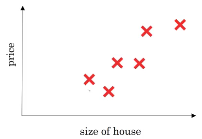
Consider an example where we have to predict the price of a house. The variables we are given are the size of the house in square feet (or square meters) and the price of the house. Now assume we have 6 houses. So first let’s pull up a plot to visualize what we’re looking at:
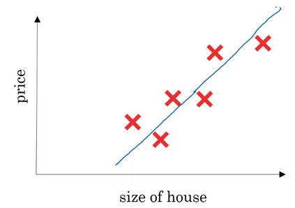
On the x-axis, we have the size of the house and on the y-axis we have it’s corresponding price. A linear regression model will try to draw a straight line to fit the data:

So, the input(x) here is the size of the house and output(y) is the price. Now let’s look at how we can solve this using a simple neural network:
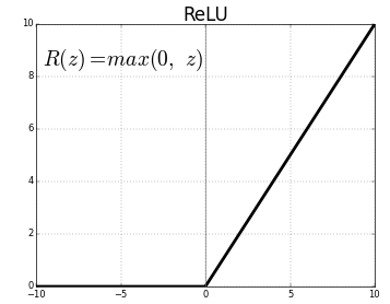
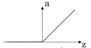
Here, a neuron will take an input, apply some activation function to it, and generate an output. One of the most commonly used activation function is ReLU (Rectified Linear Unit):
ReLU takes a real number as input and returns the maximum of 0 or that number. So, if we pass 10, the output will be 10, and if the input is -10, the output will be 0. We will discuss activation functions in detail later in this article.
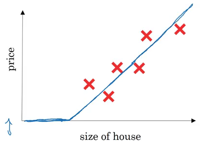
For now let’s stick to our example. If we use the ReLU activation function to predict the price of a house based on its size, this is how the predictions may look:
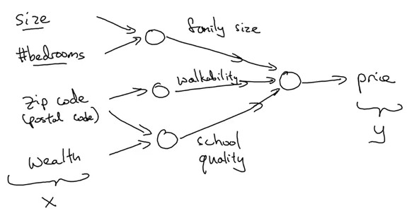
So far, we have seen a neural network with a single neuron, i.e., we only had one feature (size of the house) to predict the house price. But in reality, we’ll have to consider multiple features like number of bedrooms, postal code, etc.? House price can also depend on the family size, neighbourhood location or school quality. How can we define a neural network in such cases?
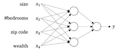
It gets a bit complicated here. Refer to the above image as you read – we pass 4 features as input to the neural network as x, it automatically identifies some hidden features from the input, and finally generates the output y. This is how a neural network with 4 inputs and an output with single hidden layer will look like:
Now that we have an intuition of what neural networks are, let’s see how we can use them for supervised learning problems.
Supervised Learning with Neural Networks
Supervised learning refers to a task where we need to find a function that can map input to corresponding outputs (given a set of input-output pairs). We have a defined output for each given input and we train the model on these examples. Below is a pretty handy table that looks at the different applications of supervised learning and the different types of neural networks that can be used to solve those problems:
| Input (X) | Output (y) | Application | Type of Neural Network |
| Home Features | Price | Real Estate | Standard Neural Network |
| Ad, user info | Click prediction (0/1) | Online Advertising | Standard Neural Network |
| Image | Image Class | Photo Tagging | CNN |
| Audio | Text Transcript | Speech Recognition | RNN |
| English | Chinese | Machine Translation | RNN |
| Image, Radar info | Position of car | Autonomous Driving | Custom / Hybrid NN |
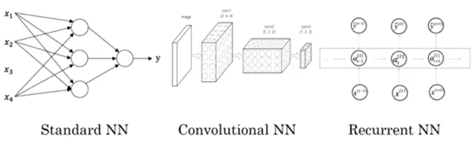
Below is a visual representation of the most common Neural Network types:
In this article, we will be focusing on the standard neural networks. Don’t worry, we will cover the other types in upcoming articles.
As you might be aware, supervised learning can be used on both structured and unstructured data.
In our house price prediction example, the given data tells us the size and the number of bedrooms. This is structured data, meaning that each feature, such as the size of the house, the number of bedrooms, etc. has a very well defined meaning.
In contrast, unstructured data refers to things like audio, raw audio, or images where you might want to recognize what’s in the image or text (like object detection). Here, the features might be the pixel values in an image, or the individual words in a piece of text. It’s not really clear what each pixel of the image represents and therefore this falls under the unstructured data umbrella.
Simple machine learning algorithms work well with structured data. But when it comes to unstructured data, their performance tends to take quite a dip. This is where neural networks have proven to be so effective and useful. They perform exceptionally well on unstructured data. Most of the ground-breaking research these days has neural networks at it’s core.
Why is Deep Learning Taking off?
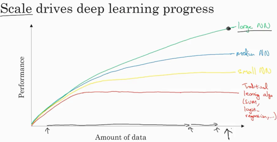
To understand this, take a look at the below graph:
As the amount of data increases, the performance of traditional learning algorithms, like SVM and logistic regression, does not improve by a whole lot. In fact, it tends to plateau after a certain point. In the case of neural networks, the performance of the model increases with an increase in the data you feed to the model.
There are basically three scales that drive a typical deep learning process:
- Data
- Computation Time
- Algorithms
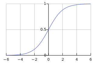
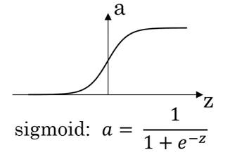
To improve the computation time of the model, activation function plays an important role. If we use a sigmoid activation function, this is what we end up with:
The slope, or the gradient of this function, at the extreme ends is close to zero. Therefore, the parameters are updated very slowly, resulting in very slow learning. Hence, switching from a sigmoid activation function to ReLU (Rectified Linear Unit) is one of the biggest breakthroughs we have seen in neural networks. ReLU updates the parameters much faster as the slope is 1 when x>0. This is the primary reason for faster computation of the models.
2.2 Module 2: Introduction to Deep Learning
The objectives behind module 2 are to:
- Build a logistic regression model, structured as a shallow neural network
- Implement the main steps of an ML algorithm, including making predictions, derivative computation, and gradient descent
- Implement computationally efficient and highly vectorized versions of models
- Understand how to compute derivatives for logistic regression, using a backpropagation mindset
- Become familiar with Python and Numpy
This module is further divided into two parts:
- Part I: Logistic Regression as a Neural Network
- Part II: Python and Vectorization
Let’s walk through each part in detail.
Part I: Logistic Regression as a Neural Network
Binary Classification
In a binary classification problem, we have an input x, say an image, and we have to classify it as having a cat or not. If it is a cat, we will assign it a 1, else 0. So here, we have only two outputs – either the image contains a cat or it does not. This is an example of a binary classification problem.
We can of course use the most popular classification technique, logistic regression, in this case.
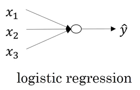
Logistic Regression
We have an input X (image) and we want to know the probability that the image belongs to class 1 (i.e. a cat). For a given X vector, the output will be:
y = w(transpose)X + b
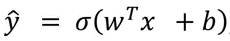
Here w and b are the parameters. Since our output y is probability, it should range between 0 and 1. But in the above equation, it can take any real value, which doesn’t make sense for getting the probability. So logistic regression also uses a sigmoid function to output probabilities:
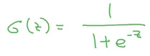
For any value as input, it will only return values in the 0 to 1 range. The formula for a sigmoid function is:
So, if z is very large, exp(-z) will be close to 0, and therefore the output of the sigmoid will be 1. Similarly, if z is very small, exp(-z) will be infinity and hence the output of the sigmoid will be 0.
Note that the parameter w is nx dimensional vector, and b is a real number. Now let’s look at the cost function for logistic regression.
Logistic Regression Cost Function
To train the parameters w and b of logistic regression, we need a cost function. We want to find parameters w and b such that at least on the training set, the outputs you have (y-hat) are close to the actual values (y).

We can use a loss function defined below:
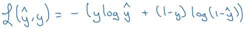
The problem with this function is that the optimization problem becomes non-convex, resulting in multiple local optima. Hence, gradient descent will not work well with this loss function. So, for logistic regression, we define a different loss function that plays a similar role as that of the above loss function and also solves the optimization problem by giving a convex function:
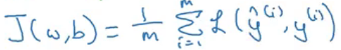
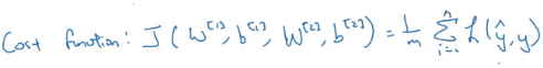
Loss function is defined for a single training example which tells us how well we are doing on that particular example. On the other hand, a cost function is for the entire training set. Cost function for logistic regression is:
We want our cost function to be as small as possible. For that, we want our parameters w and b to be optimized.
Gradient Descent
This is a technique that helps to learn the parameters w and b in such a way that the cost function is minimized. The cost function for logistic regression is convex in nature (i.e. only one global minima) and that is the reason for choosing this function instead of the squared error (can have multiple local minima).
Let’s look at the steps for gradient descent:
- Initialize w and b (usually initialized to 0 for logistic regression)
- Take a step in the steepest downhill direction
- Repeat step 2 until global optimum is achieved
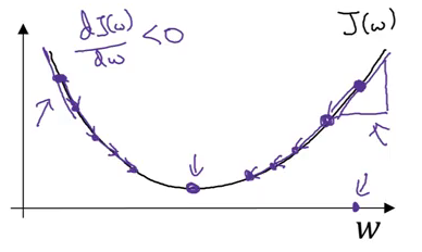
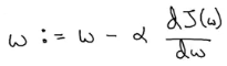
The updated equation for gradient descent becomes:
Here, ⍺ is the learning rate that controls how big a step we should take after each iteration.
If we are on the right side of the graph shown above, the slope will be positive. Using the updated equation, we will move to the left (i.e. downward direction) until the global minima is reached. Whereas if we are on the left side, the slope will be negative and hence we will take a step towards the right (downward direction) until the global minima is reached. Pretty intuitive, right?
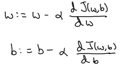
The updated equations for the parameters of logistic regression are:
Derivatives
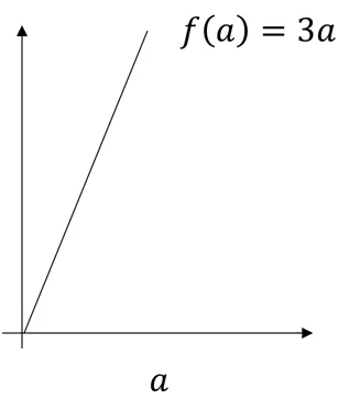
Consider a function, f(a) = 3a, as shown below:
The derivative of this function at any point will give the slope at that point. So,
f(a=2) = 3*2 = 6
f(a=2.001) = 3*2.001 = 6.003
Slope/derivative of the function at a = 2 is:
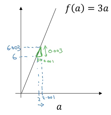
Slope = height/width
Slope = 0.003 / 0.001 = 3
This is how we calculate the derivative/slope of a function. Let’s look at a few more examples of derivatives.
More Derivative Examples
Consider the 3 functions below and their corresponding derivatives:
f(a) = a2 , d(f(a))/d(a) = 2a
f(a) = a3, d(f(a))/d(a) = 3a2
Finally, f(a) = log(a), d(f(a))/d(a) = 1/a
In all the above examples, the derivative is a function of a, which means that the slope of a function is different at different points.
Computation Graph
These graphs organize the computation of a specific function. Consider the below example:
J(a,b,c) = 3(a+bc)
We have to calculate J given a, b, and c. We can divide this into three steps:
- u = bc
- v = a+u
- J = 3v
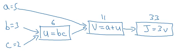
Let’s visualize these steps for a = 5, b = 3 and c = 2:
This is the forward propagation step where we have calculated the output, i.e., J. We can also use computation graphs for backward propagation where we update the parameters, a,b and c in the above example.
Derivatives with a Computation Graph
Now let’s see how we can calculate derivatives with the help of a computation graph. Suppose we have to calculate dJ/da. The steps will be:
- Since J is a function of v, calculate dJ/dv:
dJ/dv = d(3v)/dv = 3 - Since v is a function of a and u, calculate dv/da:
dv/da = d(a+u)/da = 1 - Calculate dJ/da:
dJ/da = (dJ/dv)*(dv/da) = 3*1 = 3
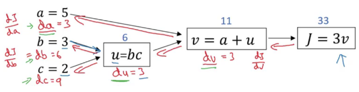
Similarly, we can calculate dJ/db and dJ/dc:
Now we will take the concept of computation graphs and gradient descent together and see how the parameters of logistic regression can be updated.
Logistic Regression Gradient Descent
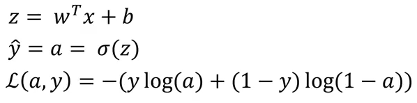
Just to quickly recap, the equations of logistic regression are:
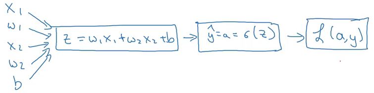
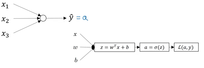
where L is the loss function. Now, for two features (x1 and x2), the computation graph for calculating the loss will be:
Here, w1, w2, and b are the parameters that need to be updated. Below are the steps to do this (for w1):
- Calculate da:
da = dL/da = (-y/a) + (1-y)/(1-a) - Calculate dz:
dz = (dL/da)*(da/dz) = [(-y/a) + (1-y)/(1-a)]*[a(1-a)] = a-y - Calculate dw1:
dw1 = [(dL/da)*(da/dz)]*dz/dw1 = (a-y)*dz/dw1
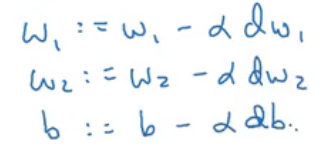
Similarly, we can calculate dw2 and db. Finally, the weights will be updated using the following equations:
Keep in mind that this is for a single training example. We will have multiple examples in real-world scenarios. So, let’s look at how gradient descent can be calculated for ‘m’ training examples.
Gradient Descent on ‘m’ Examples
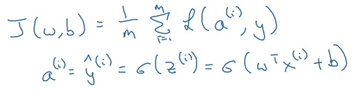
We can define the predictions and cost function for ‘m’ training examples as:

The derivative of a loss function w.r.t the parameters can be written as:
Let’s now see how we can apply logistic regression for ‘m’ examples:
J = 0; dw1 = 0; dw2 =0; db = 0;
w1 = 0; w2 = 0; b=0;
for i = 1 to m
    # Forward pass
    z(i) = W1*x1(i) + W2*x2(i) + b
    a(i) = Sigmoid(z(i))
    J += (Y(i)*log(a(i)) + (1-Y(i))*log(1-a(i)))

    # Backward pass
    dz(i) = a(i) - Y(i)
    dw1 += dz(i) * x1(i)
    dw2 += dz(i) * x2(i)
    db  += dz(i)
J /= m
dw1/= m
dw2/= m
db/= m

# Gradient descent
w1 = w1 - alpa * dw1
w2 = w2 - alpa * dw2
b = b - alpa * db
These for loops end up making the computation very slow. There is a way by which these loops can be replaced in order to make the code more efficient. We will look at these tricks in the coming sections.
Part II – Python and Vectorization
Up to this point, we have seen how to use gradient descent for updating the parameters for logistic regression. In the above example, we saw that if we have ‘m’ training examples, we have to run the loop ‘m’ number of times to get the output, which makes the computation very slow.
Instead of these for loops, we can use vectorization which is an effective and time efficient approach.
Vectorization
Vectorization is basically a way of getting rid of for loops in our code. It performs all the operations together for ‘m’ training examples instead of computing them individually. Let’s look at non-vectorized and vectorized representation of logistic regression:
Non-vectorized form:
z = 0
for i in range(nx):
   z += w[i] * x[i]
z +=b
Now, let’s look at the vectorized form. We can represent the w and x in a vector form:
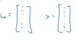
Now we can calculate Z for all the training examples using:
Z = np.dot(W,X)+b (numpy is imported as np)
The dot function of NumPy library uses vectorization by default. This is how we can vectorize the multiplications. Let’s now see how we can vectorize an entire logistic regression algorithm.
Vectorizing Logistic Regression
Keeping with the ‘m’ training examples, the first step will be to calculate Z for all of these examples:
Z = np.dot(W.T, X) + b
Here, X contains the features for all the training examples while W is the coefficient matrix for these examples. The next step is to calculate the output(A) which is the sigmoid of Z:
A = 1 / 1 + np.exp(-Z)
Now, calculate the loss and then use backpropagation to minimize the loss:
dz = A – Y
Finally, we will calculate the derivative of the parameters and update them:
dw = np.dot(X, dz.T) / m
db = dz.sum() / m
W = W – ⍺dw
b = b – ⍺db
Broadcasting in Python
Broadcasting makes certain parts of the code much more efficient. But don’t just take my word for it! Let’s look at some examples:
- obj.sum(axis = 0) sums the columns while obj.sum(axis = 1) sums the rows
- obj.reshape(1,4) changes the shape of the matrix by broadcasting the values
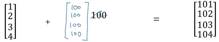
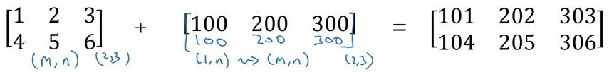
If we add 100 to a (4×1) matrix, it will copy 100 to a (4×1) matrix. Similarly, in the example below, (1×3) matrix will be copied to form a (2×3) matrix:
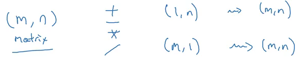
The general principle will be:
If we add, subtract, multiply or divide an (m,n) matrix with a (1,n) matrix, this will copy it m times into an (m,n) matrix. This is called broadcasting and it makes the computations much faster. Try it out yourself!
A note on Python/Numpy Vectors
If you form an array using:
a = np.random.randn(5)
It will create an array of shape (5,) which is a rank 1 array. Using this array will cause problems while taking the transpose of the array. Instead, we can use the following code to form a vector instead of a rank 1 array:
a = np.random.randn(5,1) # shape (5,1) column vector
a = np.random.randn(1,5) # shape (1,5) row vector
To convert a (1,5) row vector to a (5,1) column vector, one can use:
a = a.reshape((5,1))
That’s it for module 2. In the next section, we will dive deeper into the details of a Shallow Neural Network.
2.3 Module 3: Shallow Neural Networks
The objectives behind module 3 are to:
- Understand hidden units and hidden layers
- Be able to apply a variety of activation functions in a neural network.
- Build your first forward and backward propagation with a hidden layer
- Apply random initialization to your neural network
- Become fluent with Deep Learning notations and Neural Network Representations
- Build and train a neural network with one hidden layer
Neural Networks Overview
In logistic regression, to calculate the output (y = a), we used the below computation graph:
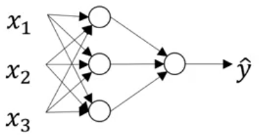
In case of a neural network with a single hidden layer, the structure will look like:
And the computation graph to calculate the output will be:
X1  \
X2   => z1 = XW1 + B1 => a1 = Sigmoid(z1) => z2 = a1W2 + B2 => a2 = Sigmoid(z2) => l(a2,Y)
X3  /
Neural Network Representation
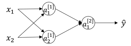
Consider the following representation of a neural network:
Can you identify the number of layers in the above neural network? Remember that while counting the number of layers in a NN, we do not count the input layer. So, there are 2 layers in the NN shown above, i.e., one hidden layer and one output layer.
The first layer is referred as a[0], second layer as a[1], and the final layer as a[2]. Here ‘a’ stands for activations, which are the values that different layers of a neural network passes on to the next layer. The corresponding parameters are w[1], b[1] and w[1], b[2]:
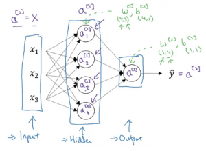
This is how a neural network is represented. Next we will look at how to compute the output from a neural network.
Computing a Neural Network’s Output
Let’s look in detail at how each neuron of a neural network works. Each neuron takes an input, performs some operation on them (calculates z = w[T] + b), and then applies the sigmoid function:
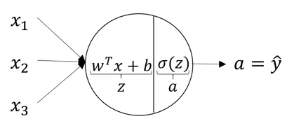
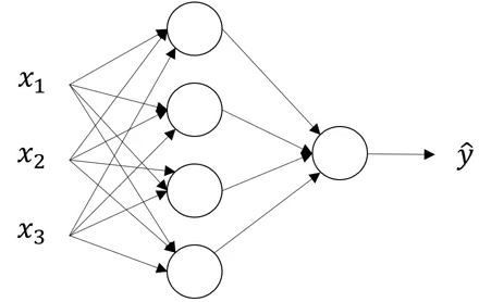
This step is performed by each neuron. The equations for the first hidden layer with four neurons will be:
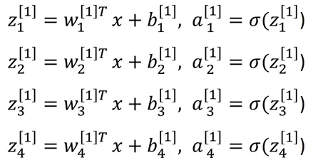
So, for given input X, the outputs for each neuron will be:
z[1] = W[1]x + b[1]
a[1] = 𝛔(z[1])
z[2] = W[2]x + b[2]
a[2] = 𝛔(z[2])
To compute these outputs, we need to run a for loop which will calculate these values individually for each neuron. But recall that using a for loop will make the computations very slow, and hence we should optimize the code to get rid of this for loop and run it faster.
Vectorizing across multiple examples
The non-vectorized form of computing the output from a neural network is:
for i=1 to m:

z[1](i) = W[1](i)x + b[1]

a[1](i) = 𝛔(z[1](i))

z[2](i) = W[2](i)x + b[2]

a[2](i) = 𝛔(z[2](i))
Using this for loop, we are calculating z and a value for each training example separately. Now we will look at how it can be vectorized. All the training examples will be merged in a single matrix X:
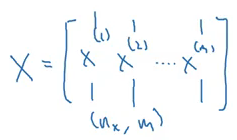
Here, nx is the number of features and m is the number of training examples. The vectorized form for calculating the output will be:
Z[1] = W[1]X + b[1]
A[1] = 𝛔(Z[1])
Z[2] = W[2]X + b[2]
A[2] = 𝛔(Z[2])
This will reduce the computation time (significantly in most cases).
Activation Function
While calculating the output, an activation function is applied. The choice of an activation function highly affects the performance of the model. So far, we have used the sigmoid activation function:
However, this might not the best option in some cases. Why? Because at the extreme ends of the graph, the derivative will be close to zero and hence the gradient descent will update the parameters very slowly.
There are other functions which can replace this activation function:
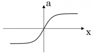
- tanh:
- ReLU (already covered earlier):
| Activation Function | Pros | Cons |
| Sigmoid | Used in the output layer for binary classification | Output ranges from 0 to 1 |
| tanh | Better than sigmoid | Updates parameters slowly when points are at extreme ends |
| ReLU | Updates parameters faster as slope is 1 when x>0 | Zero slope when x<0 |
We can choose different activation functions depending on the problem we’re trying to solve.
Why do we need non-linear activation functions?
If we use linear activation functions on the output of the layers, it will compute the output as a linear function of input features. We first calculate the Z value as:
Z = WX + b
In case of linear activation functions, the output will be equal to Z (instead of calculating any non-linear activation):
A = Z
Using linear activation is essentially pointless. The composition of two linear functions is itself a linear function, and unless we use some non-linear activations, we are not computing more interesting functions. That’s why most experts stick to using non-linear activation functions.
There is only one scenario where we tend to use a linear activation function. Suppose we want to predict the price of a house (which can be any positive real number). If we use a sigmoid or tanh function, the output will range from (0,1) and (-1,1) respectively. But the price will be more than 1 as well. In this case, we will use a linear activation function at the output layer.
Once we have the outputs, what’s the next step? We want to perform backpropagation in order to update the parameters using gradient descent.
Gradient Descent for Neural Networks
The parameters which we have to update in a two-layer neural network are: w[1], b[1], w[2] and b[2], and the cost function which we will be minimizing is:
The gradient descent steps can be summarized as:
Repeat:
    Compute predictions (y'(i), i = 1,...m)
    Get derivatives: dW[1], db[1], dW[2], db[2]
    Update: W[1] = W[1] - ⍺ * dW[1]
            b[1] = b[1] - ⍺ * db[1]
            W[2] = W[2] - ⍺ * dW[2]
            b[2] = b[2] - ⍺ * db[2]
Let’s quickly look at the forward and backpropagation steps for a two-layer neural networks.
Forward propagation:
Z[1] = W[1]*A[0] + b[1]    # A[0] is X
A[1] = g[1](Z[1])
Z[2] = W[2]*A[1] + b[2]
A[2] = g[2](Z[2])
Backpropagation:
dZ[2] = A[2] - Y
dW[2] = (dZ[2] * A[1].T) / m
db[2] = Sum(dZ[2]) / m
dZ[1] = (W[2].T * dZ[2]) * g'[1](Z[1])  # element wise product (*)
dW[1] = (dZ[1] * A[0].T) / m   # A[0] = X
db[1] = Sum(dZ[1]) / m
These are the complete steps a neural network performs to generate outputs. Note that we have to initialize the weights (W) in the beginning which are then updated in the backpropagation step. So let’s look at how these weights should be initialized.
Random Initialization
We have previously seen that the weights are initialized to 0 in case of a logistic regression algorithm. But should we initialize the weights of a neural network to 0? It’s a pertinent question. Let’s consider the example shown below:
If the weights are initialized to 0, the W matrix will be:
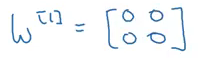
Using these weights:
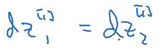
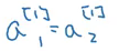
And finally at the backpropagation step:
No matter how many units we use in a layer, we are always getting the same output which is similar to that of using a single unit. So, instead of initializing the weights to 0, we randomly initialize them using the following code:
w[1] = np.random.randn((2,2)) * 0.01
b[1] = np.zero((2,1))
We multiply the weights with 0.01 to initialize small weights. If we initialize large weights, the activation will be large, resulting in zero slope (in case of sigmoid and tanh activation function). Hence, learning will be slow. So we generally initialize small weights randomly.
2.4 Module 4: Deep Neural Networks
It’s finally time to learn about deep neural networks! These have become today’s buzzword in the industry and the research field. No matter which research paper I pick up these days, there is inevitably a mention of how a deep neural network was used to power the thought process behind the study.
The objectives of our final module are to:
- See deep neural networks as successive blocks put one after each other
- Build and train a deep L-layer Neural Network
- Analyze matrix and vector dimensions to check neural network implementations
- Understand how to use a cache to pass information from forward propagation to backpropagation
- Understand the role of hyperparameters in deep learning
Deep L-Layer Neural Network
In this section, we will look at how the concepts of forward and backpropogation can be applied to deep neural networks. But you might be wondering at this point what in the world deep neural networks actually are?
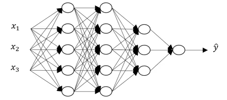
Shallow vs depth is a matter of degree. A logistic regression is a very shallow model as it has only one layer (remember we don’t count the input as a layer):
A deeper neural network has more number of hidden layers:
Let’s look at some of the notations related to deep neural networks:
- L is the number of layers in the neural network
- n[l] is the number of units in layer l
- a[l] is the activations in layer l
- w[l] is the weights for z[l]
These are some of the notations which we will be using in the upcoming sections. Keep them in mind as we proceed, or just quickly hop back here in case you miss something.
Forward Propagation in a Deep Neural Network
For a single training example, the forward propagation steps can be written as:
z[l] = W[l]a[l-1] + b[l]
a[l] = g[l](z[l])
We can vectorize these steps for ‘m’ training examples as shown below:
Z[l] = W[l]A[l-1] + B[l]
A[l] = g[l](Z[l])
These outputs from one layer act as an input for the next layer. We can’t compute the forward propagation for all the layers of a neural network without a for loop, so its fine to have a for loop here. Before moving further, let’s look at the dimensions of various matrices that will help us understand these steps in a better way.
Getting your matrix dimensions right
Analyzing the dimensions of a matrix is one of the best debugging tools to check how correct our code is. We will discuss what should be the correct dimension for each matrix in this section. Consider the following example:
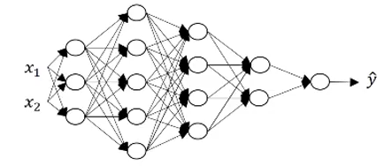
Can you figure out the number of layers (L) in this neural network? You are correct if you guessed 5. There are 4 hidden layers and 1 output layer. The units in each layer are:
n[0] = 2, n[1] = 3, n[2] = 5, n[3] = 4, n[4] = 2, and n[5] = 1
The generalized form of dimensions of W, b and their derivatives is:
- W[l] = (n[l], n[l-1])
- b[l] = (n[l], 1)
- dW[l] = (n[l], n[l-1])
- db[l] = (n[l],1)
- Dimension of Z[l], A[l], dZ[l], dA[l] = (n[l],m)
where ‘m’ is the number of training examples. These are some of the generalized matrix dimensions which will help you to run your code smoothly.
We have seen some of the basics of deep neural networks up to this point. But why do we need deep representations in the first place? Why make things complex when easier solutions exist? Let’s find out!
Why Deep Representations?
In deep neural networks, we have a large number of hidden layers. What are these hidden layers actually doing? To understand this, consider the below image:

Deep neural networks find relations with the data (simpler to complex relations). What the first hidden layer might be doing, is trying to find simple functions like identifying the edges in the above image. And as we go deeper into the network, these simple functions combine together to form more complex functions like identifying the face. Some of the common examples of leveraging a deep neural network are:
- Face Recognition
- Image ==> Edges ==> Face parts ==> Faces ==> desired face
- Audio recognition
- Audio ==> Low level sound features like (sss, bb) ==> Phonemes ==> Words ==> Sentences
Building Blocks of Deep Neural Networks
Consider any layer in a deep neural network. The input to this layer will be the activations from the previous layer (l-1), and the output of this layer will be its own activations.
- Input: a[l-1]
- Output: a[l]
This layer first calculates the z[l] on which the activations are applied. This z[l] is saved as cache. For the backward propagation step, it will first calculate da[l], i.e., derivative of the activation at layer l, derivative of weights dw[l], db[l], dz[l], and finally da[l-1]. Let’s visualize these steps to reduce the complexity:
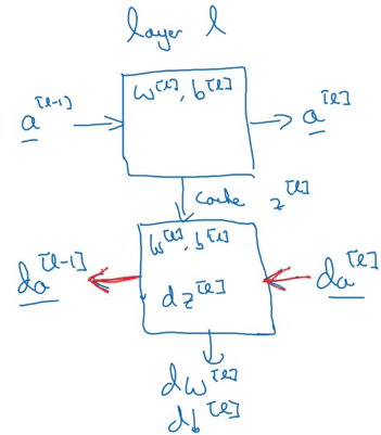
This is how each block (layer) of a deep neural network works. Next, we will see how to implement all of these blocks.
Forward and Backward Propagation
The input in a forward propagation step is a[l-1] and the outputs are a[l] and cache z[l], which is a function of w[l] and b[l]. So, the vectorized form to calculate Z[l] and A[l] is:
Z[l] = W[l] * A[l-1] + b[l]
A[l] = g[l](Z[l])
We will calculate Z and A for each layer of the network. After calculating the activations, the next step is backward propagation, where we update the weights using the derivatives. The input for backward propagation is da[l] and the outputs are da[l-1], dW[l] and db[l]. Let’s look at the vectorized equations for backward propagation:
dZ[l] = dA[l] * g'[l](Z[l])
dW[l] = 1/m * (dZ[l] * A[l-1].T)
db[l] = 1/m * np.sum(dZ[l], axis = 1, keepdims = True)

dA[l-1] = w[l].T * dZ[l]
This is how we implement deep neural networks.
Deep Neural Networks perform surprisingly well (maybe not so surprising if you’ve used them before!). Running only a few lines of code gives us satisfactory results. This is because we are feeding a large amount of data to the network and it is learning from that data using the hidden layers.
Choosing the right hyperparameters helps us to make our model more efficient. We will cover the details of hyperparameter tuning in the next article of this series.
Parameters vs Hyperparameters
This is an oft-asked question by deep learning newcomers. The major difference between parameters and hyperparameters is that parameters are learned by the model during the training time, while hyperparameters can be changed before training the model.
Parameters of a deep neural network are W and b, which the model updates during the backpropagation step. On the other hand, there are a lot of hyperparameters for a deep NN, including:
- Learning rate – ⍺
- Number of iterations
- Number of hidden layers
- Units in each hidden layer
- Choice of activation function
This was a brief overview of the difference between these two aspects. I am happy to answer any questions you might have about this, in the comments section below.
End Notes
Congrats for completing the first course in this specialization! We now know how to implement forward and backward propagation and gradient descent for deep neural networks. We have also seen how vectorization helps us to get rid of explicit for loops, making our code efficient in the process.
In the next article (which will cover course #2), we will see how we can improve deep neural networks by hyperparameter tuning, regularization and optimization. It’s one of the more tricky and fascinating aspects of deep learning.
If you have any feedback or have any doubts/questions, please feel free to share them in the comments section below. I look forward to hearing your thoughts!
To deepen your understanding, explore the detailed working of neural networks in our next module.
backward propagationdeep learningDeep Neural NetworkForward Propagationgradient descentneural networks
Pulkit Sharma
12 Jul, 2024
My research interests lies in the field of Machine Learning and Deep Learning. Possess an enthusiasm for learning new skills and technologies.


Brilliant article, thank yoU!
Thank you Hayden!
On my opinion. This is one of the best posts and explanations about neural networks. It doesn't go too deep into maths but is not shallow either which shows you a really good starting point for dive deeper into NN in the future course #2. Thanks so much for your effort Pulkit! can't wait to read the second course!. Regards.
Thank you Alfonso! Will be publishing the second article of this series soon.
Thank you very. Very nice explanation of ANN.
Thank you Shiam!
A nice and concise read of the concepts around different types of Neural Networks.
Hi Priyajeev, Glad you liked it!
If you can teach it, you've mastered it. Congratulations!
Thank you Nick!
Excellent tutorial. I have taken this course previously but reading your article just helped to improve my understanding a lot more. Thanks a lot!
Hi, Glad you found it helpful.
Just started with this course today, thanks for this beautiful insight bro :)
Thank you Gaurav!
Fantastic Explanation. Just loved it. Excellent.
Glad you liked it Somanath!
Excellent. I did the specialization and hoped there would be a kind of handbook for the courses. As this was not the case I had to hurry downloading the slides. Will these notes be available in downloadable format (PDF etc.) in the future?
Hi Michael, Right now we do not have an option to download these articles. Whereas, in the future, there will be a feature which will help you to download these articles.
A very insightful and easy-to-understand article. When will the next article be available?
Thank you Ibrahim! I am currently working on it and will publish the next article shortly.
I just completed the article. This is what I call easy explanation for easy learning. Thank you so much for creating this. Waiting for the course #2
Glad you liked it Abhijit! I am currently working on course #2 and will publish it shortly.
Earnestly waiting for Course 2. Thank you sir.
Thank you Ibrahim! The second part will be released soon.
Hi PULKIT, Thanks for the 101 on Deep Learning, which alot of people dont usually delve into especially when there is alot of equations. But yours was smoothly touching the surface. Just double checking with good-self, maybe there is a typo error at para : --Extracts-- Forward Propagation in a Deep Neural Network For a single training example, the forward propagation steps can be written as: z[l] = W[l]a[l-1] + b[l] a[l] = g[l](a[l]) <-- shud be g[l](z[l]) Z[l] = W[l]A[l-1] + B[l] A[l] = g[l](A[l]) <-- shud be g[l](Z[l]) Will go into your part 2 soon. Thanks once again.
Hi Zarief, Thanks for pointing it out. Have updated it in the article.
Hi Pulkit, it a great refresher !
Good explanation. Where can I get the implementation of the above code? Is it hosted in Github?
Hi Prakash, You can find them here.
Incredible .. Thank you so much. Please keep going .. Looking forward for more articles.
Thanks you Ebtihal. I have written notes on other courses of deep learning specialization as well. Feel free to check them out: Course 2 Course 4 Course 5
Dear pulkit....awesome I can say..ppl like who want to get into ML and DL it helps..can you tell me I can say is this a starting point or I do required python knowledge
Thanks PULKIT SHARMA for these notes. I find them very clear and useful. However, I have been asking myself many times that, how activation functions like Relu, Leaky Relu, Tanh, etc., when being put into the deep neural network, can give such an accurate output to predict human behavior? What is the relationship between activation functions and human behavior? Is that the law of the universe, law of god, or something magic that cannot be explained clearly now? Furthermore, the explanation about Deep Representation, however, does not give me a clear intuition, how pixels being put into activation functions in many layers, then finally can show it is a cat or a dog? I look forward to your answers to my 2 questions, or any readings to clarify my doubts. Thank you very much! Wish you good health and success.
Hi Dat, Glad you liked this post. Activation functions are one of the most important element of any neural network, whether it be ANNs or CNNs. They eventually decides whether a neuron should activate or not. I would recommend you to go through this article which will give you a better understanding of why activation functions are important and how can they help you to build a model equivalent to human behavior.
Hi Pulkit, Great tutorial! But I have a doubt. I might be missing something so please guide: L(a,y) = - (ylog(a) + (1-y)log(1-a)), then Calculate da: da = dL/da = (-y/a) + (1-y)/(1-a) Calculate dz: dz = (dL/da)*(da/dz) = [(-y/a) + (1-y)/(1-a)]*[a(1-a)] = a-y My doubt is, since the -ve sign in loss function is outside of the braces, wouldn't the value of "da" be -(y/a) -(1-y)/(1-a) ? Sorry, if that is a stupid question but kindly guide Thanks
Hi Karan, The derivative of log(1-a) will be [1/(1-a)]*(-1) and hence the final value will be -(y/a) -[(1-y)/(1-a)]*(-1) = -(y/a) + (1-y)/(1-a)
Hi Pulkit, Thank you for the Great tutorial! I have a doubt in Logistic Regression Gradient Descent. When loss function is: L(a,y) = - (ylog(a) + (1-y)log(1-a)), we found da = dL/da = (-y/a) + (1-y)/(1-a) But since the -ve sign in loss function is outside of the braces, wouldn't da = - (y/a) - (1-y)/(1-a) ? Please guide Thanks, Karan
Very well explained Thank you for the great effort!!!!!
Incredible .. Thank you so much. Please keep going .. Looking forward for more articles
Very well explained Thank you
Good Traning Introductory Guide to Deep Learning and Neural Networks
Very well explained Thank you
Good Traning Introductory Guide to Deep Learning and Neural Networks
Very well explained Thank you
Very well explained Thank you.
it is very helpful to understand