Introduction
PyTorch v TensorFlow – how many times have you seen this polarizing question pop up on social media? The rise of deep learning in recent times has been fuelled by the popularity of these frameworks. There are staunch supporters of both, but a clear winner has started to emerge in the last year.
PyTorch was one of the most popular frameworks in 2018. It quickly became the preferred go-to deep learning framework among researchers in both academia and the industry. After using PyTorch for the last few weeks, I can confirm that it is highly flexible and an easy-to-use deep learning library.
In this article, we will explore what PyTorch is all about. But our learning won’t stop with the theory – we will code through 4 different use cases and see how well PyTorch performs. Building deep learning models has never been this fun!
Note: This article assumes that you have a basic understanding of deep learning concepts. If not, I recommend going through this article.
If you prefer to approach the following concepts in a structured format, you can enrol for this free course on PyTorch and follow them chapter-wise.
Contents
- What is PyTorch?
- Building Neural Nets using PyTorch
- Use Case 1: Handwritten Digits Classification (Numerical Data, MLP)
- Use Case 2: Objects Image Classification (Image Data, CNN)
- Use Case 3: Sentiment Text Classification (Text Data, RNN)
- Use Case 4: Image Style Transfer (Transfer Learning)
What is PyTorch?
Let’s understand what PyTorch is and why it has become so popular lately, before diving into it’s implementation.
PyTorch is a Python-based scientific computing package that is similar to NumPy, but with the added power of GPUs. It is also a deep learning framework that provides maximum flexibility and speed during implementing and building deep neural network architectures.
Recently, PyTorch 1.0 was released and it was aimed to assist researchers by addressing four major challenges:
- Extensive reworking
- Time-consuming training
- Python programming language inflexibility
- Slow scale-up
Intrinsically, there are two main characteristics of PyTorch that distinguish it from other deep learning frameworks like Tensorflow:
- Imperative Programming
- Dynamic Computation Graphing
Imperative Programming: PyTorch performs computations as it goes through each line of the written code. This is quite similar to how a Python program is executed. This concept is called imperative programming. The biggest advantage of this feature is that your code and programming logic can be debugged on the fly.
Dynamic Computation Graphing: PyTorch is referred to as a “defined by run” framework, which means that the computational graph structure (of a neural network architecture) is generated during run time. The main advantage of this property is that it provides a flexible and programmatic runtime interface that facilitates the construction and modification of systems by connecting operations. In PyTorch, a new computational graph is defined at each forward pass. This is in stark contrast to TensorFlow which uses a static graph representation.
PyTorch 1.0 comes with an important feature called torch.jit, a high-level compiler that allows the user to separate the models and code. It also supports efficient model optimization on custom hardware, such as GPUs or TPUs.
Building Neural Nets using PyTorch
Let’s understand PyTorch through a more practical lens. Learning theory is good, but it isn’t much use if you don’t put it into practice!
A PyTorch implementation of a neural network looks exactly like a NumPy implementation. The goal of this section is to showcase the equivalent nature of PyTorch and NumPy. For this purpose, let’s create a simple three-layered network having 5 nodes in the input layer, 3 in the hidden layer, and 1 in the output layer. We will use only one training example with one row which has five features and one target.
import torch
n_input, n_hidden, n_output = 5, 3, 1
The first step is to do parameter initialization. Here, the weights and bias parameters for each layer are initialized as the tensor variables. Tensors are the base data structures of PyTorch which are used for building different types of neural networks. They can be considered as the generalization of arrays and matrices; in other words, tensors are N-dimensional matrices.
## initialize tensor for inputs, and outputs
x = torch.randn((1, n_input))
y = torch.randn((1, n_output))
## initialize tensor variables for weights
w1 = torch.randn(n_input, n_hidden) # weight for hidden layer
w2 = torch.randn(n_hidden, n_output) # weight for output layer
## initialize tensor variables for bias terms
b1 = torch.randn((1, n_hidden)) # bias for hidden layer
b2 = torch.randn((1, n_output)) # bias for output layer
After the parameter initialization step, a neural network can be defined and trained in four key steps:
- Forward Propagation
- Loss computation
- Backpropagation
- Updating the parameters
Let’s see each of these steps in a bit more detail.
Forward Propagation: In this step, activations are calculated at every layer using the two steps shown below. These activations flow in the forward direction from the input layer to the output layer in order to generate the final output.
- z = weight * input + bias
- a = activation_function (z)
The following code blocks show how we can write these steps in PyTorch. Notice that most of the functions, such as exponential and matrix multiplication, are similar to the ones in NumPy.
## sigmoid activation function using pytorch
def sigmoid_activation(z):
    return 1 / (1 + torch.exp(-z))
## activation of hidden layer
z1 = torch.mm(x, w1) + b1
a1 = sigmoid_activation(z1)
## activation (output) of final layer
z2 = torch.mm(a1, w2) + b2
output = sigmoid_activation(z2)
Loss Computation: In this step, the error (also called loss) is calculated in the output layer. A simple loss function can tell the difference between the actual value and the predicted value. Later, we will look at different loss functions available in PyTorch.
loss = y - output
Backpropagation: The aim of this step is to minimize the error in the output layer by making marginal changes in the bias and the weights. These marginal changes are computed using the derivatives of the error term.
Based on the Calculus principle of the Chain rule, the delta changes are back passed to hidden layers where corresponding changes in their weights and bias are made. This leads to an adjustment in the weights and bias until the error is minimized.
## function to calculate the derivative of activation
def sigmoid_delta(x):
  return x * (1 - x)
## compute derivative of error terms
delta_output = sigmoid_delta(output)
delta_hidden = sigmoid_delta(a1)
## backpass the changes to previous layers
d_outp = loss * delta_output
loss_h = torch.mm(d_outp, w2.t())
d_hidn = loss_h * delta_hidden
Updating the Parameters: Finally, the weights and bias are updated using the delta changes received from the above backpropagation step.
learning_rate = 0.1
w2 += torch.mm(a1.t(), d_outp) * learning_rate
w1 += torch.mm(x.t(), d_hidn) * learning_rate
b2 += d_outp.sum() * learning_rate
b1 += d_hidn.sum() * learning_rate
Finally, when these steps are executed for a number of epochs with a large number of training examples, the loss is reduced to a minimum value. The final weight and bias values are obtained which can then be used to make predictions on the unseen data.
Use Case 1: Handwritten Digital Classification
In the previous section, we saw a simple use case of PyTorch for writing a neural network from scratch. In this section, we will use different utility packages provided within PyTorch (nn, autograd, optim, torchvision, torchtext, etc.) to build and train neural networks.
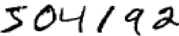
Neural networks can be defined and managed easily using these packages. In our use case, we will create a Multi-Layered Perceptron (MLP) network for building a handwritten digit classifier. We will make use of the MNIST dataset included in the torchvision package.
The first step, as with any project you’ll work on, is data preprocessing. We need to transform the raw dataset into tensors and normalize them in a fixed range. The torchvision package provides a utility called transforms which can be used to combine different transformations together.
from torchvision import transforms
_tasks = transforms.Compose([
    transforms.ToTensor(),
    transforms.Normalize((0.5, 0.5, 0.5), (0.5, 0.5, 0.5))
    ])
The first transformation converts the raw data into tensor variables and the second transformation performs normalization using the below operation:
x_normalized = x-mean / std
The values 0.5 and 0.5 represent the mean and standard deviation for 3 channels: red, green, and blue.
from torchvision.datasets import MNIST
## Load MNIST Dataset and apply transformations
mnist = MNIST("data", download=True, train=True, transform=_tasks)
Another excellent utility of PyTorch is DataLoader iterators which provide the ability to batch, shuffle and load the data in parallel using multiprocessing workers. For the purpose of evaluating our model, we will partition our data into training and validation sets.
from torch.utils.data import DataLoader
from torch.utils.data.sampler import SubsetRandomSampler
## create training and validation split
split = int(0.8 * len(mnist))
index_list = list(range(len(mnist)))
train_idx, valid_idx = index_list[:split], index_list[split:]
## create sampler objects using SubsetRandomSampler
tr_sampler = SubsetRandomSampler(train_idx)
val_sampler = SubsetRandomSampler(valid_idx)
## create iterator objects for train and valid datasets
trainloader = DataLoader(mnist, batch_size=256, sampler=tr_sampler)
validloader = DataLoader(mnist, batch_size=256, sampler=val_sampler)
The neural network architectures in PyTorch can be defined in a class which inherits the properties from the base class from nn package called Module. This inheritance from the nn.Module class allows us to implement, access, and call a number of methods easily. We can define all the layers inside the constructor of the class, and the forward propagation steps inside the forward function.
We will define a network with the following layer configurations: [784, 128,10]. This configuration represents the 784 nodes (28*28 pixels) in the input layer, 128 in the hidden layer, and 10 in the output layer. Inside the forward function, we will use the sigmoid activation function in the hidden layer (which can be accessed from the nn module).
import torch.nn.functional as F
class Model(nn.Module):
    def __init__(self):
        super().__init__()
        self.hidden = nn.Linear(784, 128)
        self.output = nn.Linear(128, 10)

   def forward(self, x):
        x = self.hidden(x)
        x = F.sigmoid(x)
        x = self.output(x)
        return x
model = Model()
Define the loss function and the optimizer using the nn and optim package:
from torch import optim
loss_function = nn.CrossEntropyLoss()
optimizer = optim.SGD(model.parameters(), lr=0.01, weight_decay= 1e-6, momentum = 0.9, nesterov = True)
We are now ready to train the model. The core steps will remain the same as we saw earlier: Forward Propagation, Loss Computation, Backpropagation, and updating the parameters.
for epoch in range(1, 11): ## run the model for 10 epochs
    train_loss, valid_loss = [], []
    ## training part
    model.train()
    for data, target in trainloader:
        optimizer.zero_grad()
        ## 1. forward propagation
        output = model(data)

        ## 2. loss calculation
        loss = loss_function(output, target)

        ## 3. backward propagation
        loss.backward()

        ## 4. weight optimization
        optimizer.step()

        train_loss.append(loss.item())

    ## evaluation part
    model.eval()
    for data, target in validloader:
        output = model(data)
        loss = loss_function(output, target)
        valid_loss.append(loss.item())
print ("Epoch:", epoch, "Training Loss: ", np.mean(train_loss), "Valid Loss: ", np.mean(valid_loss))
>> Epoch: 1  Training Loss:  0.645777 Valid Loss:  0.344971
>> Epoch: 2  Training Loss:  0.320241 Valid Loss:  0.299313
>> Epoch: 3  Training Loss:  0.278429 Valid Loss:  0.269018
>> Epoch: 4  Training Loss:  0.246289 Valid Loss:  0.237785
>> Epoch: 5  Training Loss:  0.217010 Valid Loss:  0.217133
>> Epoch: 6  Training Loss:  0.193017 Valid Loss:  0.206074
>> Epoch: 7  Training Loss:  0.174385 Valid Loss:  0.180163
>> Epoch: 8  Training Loss:  0.157574 Valid Loss:  0.170064
>> Epoch: 9  Training Loss:  0.144316 Valid Loss:  0.162660
>> Epoch: 10 Training Loss:  0.133053 Valid Loss:  0.152957
Once the model is trained, make the predictions on the validation data.
## dataloader for validation dataset
dataiter = iter(validloader)
data, labels = dataiter.next()
output = model(data)
_, preds_tensor = torch.max(output, 1)
preds = np.squeeze(preds_tensor.numpy())
print ("Actual:", labels[:10])
print ("Predicted:", preds[:10])
>>> Actual: [0 1 1 1 2 2 8 8 2 8]
>>> Predicted: [0 1 1 1 2 2 8 8 2 8]
Use Case 2: Object Image Classification
Let’s take things up a notch.
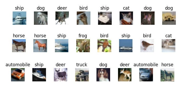
In this use case, we will create convolutional neural network (CNN) architectures in PyTorch. We will perform object image classification using the popular CIFAR-10 dataset. This dataset is also included in the torchvision package. The entire procedure to define and train the model will remain the same as the previous use case, except the introduction of additional layers in the network.
Let’s load and transform the dataset:
## load the dataset
from torchvision.datasets import CIFAR10
cifar = CIFAR10('data', train=True, download=True, transform=_tasks)
## create training and validation split
split = int(0.8 * len(cifar))
index_list = list(range(len(cifar)))
train_idx, valid_idx = index_list[:split], index_list[split:]
## create training and validation sampler objects
tr_sampler = SubsetRandomSampler(train_idx)
val_sampler = SubsetRandomSampler(valid_idx)
## create iterator objects for train and valid datasets
trainloader = DataLoader(cifar, batch_size=256, sampler=tr_sampler)
validloader = DataLoader(cifar, batch_size=256, sampler=val_sampler)
We will create the architecture with three convolutional layers for low-level feature extraction, three pooling layers for maximum information extraction, and two linear layers for linear classification.
class Model(nn.Module):
    def __init__(self):
        super(Model, self).__init__()

        ## define the layers
        self.conv1 = nn.Conv2d(3, 16, 3, padding=1)
        self.conv2 = nn.Conv2d(16, 32, 3, padding=1)
        self.conv3 = nn.Conv2d(32, 64, 3, padding=1)
        self.pool = nn.MaxPool2d(2, 2)
        self.linear1 = nn.Linear(1024, 512)
        self.linear2 = nn.Linear(512, 10)

    def forward(self, x):
        x = self.pool(F.relu(self.conv1(x)))
        x = self.pool(F.relu(self.conv2(x)))
        x = self.pool(F.relu(self.conv3(x)))
        x = x.view(-1, 1024) ## reshaping
        x = F.relu(self.linear1(x))
        x = self.linear2(x)
        return x

model = Model()
Define the loss function and the optimizer:
import torch.optim as optim
loss_function = nn.CrossEntropyLoss()
optimizer = optim.SGD(model.parameters(), lr=0.01, weight_decay= 1e-6, momentum = 0.9, nesterov = True)
## run for 30 Epochs
for epoch in range(1, 31):
    train_loss, valid_loss = [], []
    ## training part
    model.train()
    for data, target in trainloader:
        optimizer.zero_grad()
        output = model(data)
        loss = loss_function(output, target)
        loss.backward()
        optimizer.step()
        train_loss.append(loss.item())

    ## evaluation part
    model.eval()
    for data, target in validloader:
        output = model(data)
        loss = loss_function(output, target)
        valid_loss.append(loss.item())
Once the model is trained, we can generate predictions on the validation set.
## dataloader for validation dataset
dataiter = iter(validloader)
data, labels = dataiter.next()
output = model(data)
_, preds_tensor = torch.max(output, 1)
preds = np.squeeze(preds_tensor.numpy())
print ("Actual:", labels[:10])
print ("Predicted:", preds[:10])
Actual: ['truck', 'truck', 'truck', 'horse', 'bird', 'truck', 'ship', 'bird', 'deer', 'bird']
Pred:   ['truck', 'automobile', 'automobile', 'horse', 'bird', 'airplane', 'ship', 'bird', 'deer', 'bird']
Use Case 3: Sentiment Text Classification
We’ll pivot from computer vision use cases to natural language processing. The idea is to showcase the utility of PyTorch in a variety of domains in deep learning.
In this section, we’ll leverage PyTorch for text classification tasks using RNN (Recurrent Neural Networks) and LSTM (Long Short Term Memory) layers. First, we will load a dataset containing two fields — text and target. The target contains two classes, class1 and class2, and our task is to classify each text into one of these classes.
You can download the dataset here.
train = pd.read_csv("train.csv")
x_train = train["text"].values
y_train = train['target'].values
I highly recommend setting seeds before getting into the heavy coding. This ensures that the results you will see are the same as mine – a very useful (and helpful) feature when learning new concepts.
np.random.seed(123)
torch.manual_seed(123)
torch.cuda.manual_seed(123)
torch.backends.cudnn.deterministic = True
In the preprocessing step, convert the text data into a padded sequence of tokens so that it can be passed into embedding layers. I will use the utilities provided in the Keras package, but the same can be done using the torchtext package as well.
from keras.preprocessing import text, sequence
## create tokens
tokenizer = Tokenizer(num_words = 1000)
tokenizer.fit_on_texts(x_train)
word_index = tokenizer.word_index
## convert texts to padded sequences
x_train = tokenizer.texts_to_sequences(x_train)
x_train = pad_sequences(x_train, maxlen = 70)
Next, we need to convert the tokens into vectors. I will use pretrained GloVe word embeddings for this purpose. We will load these word embeddings and create an embedding matrix containing the word vector for every word in the vocabulary.
EMBEDDING_FILE = 'glove.840B.300d.txt'
embeddings_index = {}
for i, line in enumerate(open(EMBEDDING_FILE)):
    val = line.split()
    embeddings_index[val[0]] = np.asarray(val[1:], dtype='float32')
embedding_matrix = np.zeros((len(word_index) + 1, 300))
for word, i in word_index.items():
    embedding_vector = embeddings_index.get(word)
    if embedding_vector is not None:
        embedding_matrix[i] = embedding_vector
Define the model architecture with embedding layers and LSTM layers:
class Model(nn.Module):
    def __init__(self):
        super(Model, self).__init__()

        ## Embedding Layer, Add parameter
        self.embedding = nn.Embedding(max_features, embed_size)
        et = torch.tensor(embedding_matrix, dtype=torch.float32)
        self.embedding.weight = nn.Parameter(et)
        self.embedding.weight.requires_grad = False
        self.embedding_dropout = nn.Dropout2d(0.1)
        self.lstm = nn.LSTM(300, 40)
        self.linear = nn.Linear(40, 16)
        self.out = nn.Linear(16, 1)
        self.relu = nn.ReLU()
   def forward(self, x):
        h_embedding = self.embedding(x)
        h_lstm, _ = self.lstm(h_embedding)
        max_pool, _ = torch.max(h_lstm, 1)
        linear = self.relu(self.linear(max_pool))
        out = self.out(linear)
        return out
model = Model()
Create training and validation sets:
from torch.utils.data import TensorDataset
## create training and validation split
split_size = int(0.8 * len(train_df))
index_list = list(range(len(train_df)))
train_idx, valid_idx = index_list[:split], index_list[split:]
## create iterator objects for train and valid datasets
x_tr = torch.tensor(x_train[train_idx], dtype=torch.long)
y_tr = torch.tensor(y_train[train_idx], dtype=torch.float32)
train = TensorDataset(x_tr, y_tr)
trainloader = DataLoader(train, batch_size=128)
x_val = torch.tensor(x_train[valid_idx], dtype=torch.long)
y_val = torch.tensor(y_train[valid_idx], dtype=torch.float32)
valid = TensorDataset(x_val, y_val)
validloader = DataLoader(valid, batch_size=128)
Define loss and optimizers:
loss_function = nn.BCEWithLogitsLoss(reduction='mean')
optimizer = optim.Adam(model.parameters())
Training the model:
## run for 10 Epochs
for epoch in range(1, 11):
    train_loss, valid_loss = [], []
## training part
    model.train()
    for data, target in trainloader:
        optimizer.zero_grad()
        output = model(data)
        loss = loss_function(output, target.view(-1,1))
        loss.backward()
        optimizer.step()
        train_loss.append(loss.item())

    ## evaluation part
    model.eval()
    for data, target in validloader:
        output = model(data)
        loss = loss_function(output, target.view(-1,1))
        valid_loss.append(loss.item())
Finally, we can obtain the predictions:
dataiter = iter(validloader)
data, labels = dataiter.next()
output = model(data)
_, preds_tensor = torch.max(output, 1)
preds = np.squeeze(preds_tensor.numpy())
Actual: [0 1 1 1 1 0 0 0 0]
Predicted: [0 1 1 1 1 1 1 1 0 0]
Use Case #4: Image Style Transfer
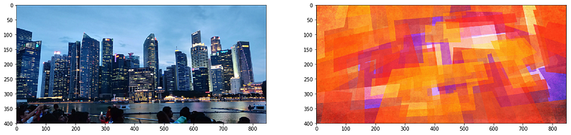
Let’s look at one final use case where we will perform artistic style transfer. This is one of the most creative projects I have worked on and hopefully you’ll have fun with this as well. The basic idea behind the style transfer concept is:
- Take the objects/context from one image
- Take the style/texture from a second image
- Generate a final image which is a mixture of the two
This concept was introduced in the paper: “Image Style Transfer using Convolutional Networks”. An example of style transfer is shown below:
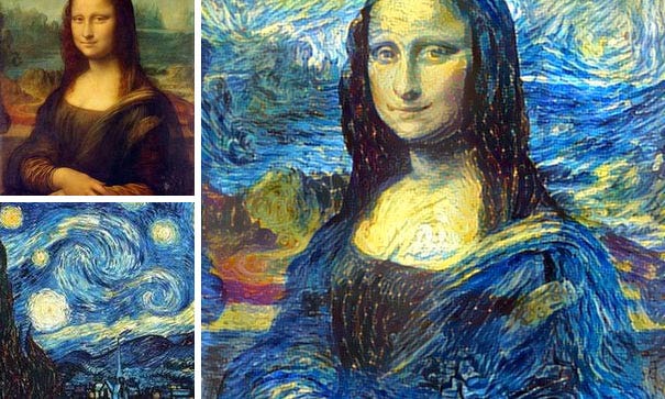
Awesome, right? Let’s look at it’s implementation in PyTorch. The process involves six steps:
- Low-level feature extraction from both the input images. This can be done using pretrained deep learning models such as VGG19.
from torchvision import models
# get the features portion from VGG19
vgg = models.vgg19(pretrained=True).features

# freeze all VGG parameters
for param in vgg.parameters():
    param.requires_grad_(False)
# check if GPU is available
device = torch.device("cpu")
if torch.cuda.is_available():
    device = torch.device("cuda")
vgg.to(device)
- Load the two images on the device and obtain the features from VGG. Also, apply the transformations: resize to tensor, and normalization of values.
from torchvision import transforms as tf
def transformation(img):
    tasks = tf.Compose([tf.Resize(400), tf.ToTensor(),
               tf.Normalize((0.44,0.44,0.44),(0.22,0.22,0.22))])
    img = tasks(img)[:3,:,:].unsqueeze(0)
    return img
img1 = Image.open("image1.jpg").convert('RGB')
img2 = Image.open("image2.jpg").convert('RGB')
img1 = transformation(img1).to(device)
img2 = transformation(img2).to(device)
- Now, we need to obtain the relevant features of the two images. From the first image, we need to extract features related to the context or the objects present. From the second image, we need to extract features related to styles and textures.
Object Related Features: In the original paper, the authors have suggested that more valuable information about objects and context can be extracted from the initial layers of the network. This is because in the higher layers, the information space becomes more complex and detailed pixel information is lost.
Style Related Features: In order to obtain the texture information from the second image, the authors used correlations between different features in different layers. This is explained in detail in point 4 below.
But before getting there, let’s look at the structure of a typical VGG19 model:
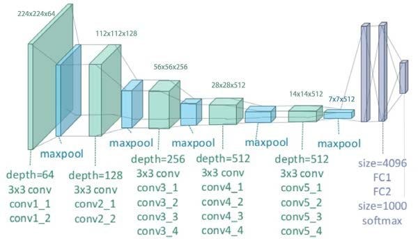
For object information extraction, Conv42 was the layer of interest. It’s present in the 4th convolutional block with a depth of 512. For style representation, the layers of interest were the first convolutional layer of every convolutional block in the network, i.e., conv11, conv21, conv31, conv41, and conv51. These layers were selected purely based on the author’s experiments and I am only replicating their results in this article.
def get_features(image, model):
    layers = {'0': 'conv1_1', '5': 'conv2_1',  '10': 'conv3_1',
              '19': 'conv4_1', '21': 'conv4_2', '28': 'conv5_1'}
    x = image
    features = {}
    for name, layer in model._modules.items():
        x = layer(x)
        if name in layers:
            features[layers[name]] = x
    return features
img1_features = get_features(img1, vgg)
img2_features = get_features(img2, vgg)
- As mentioned in the previous point, the authors used correlations in different layers to obtain the style related features. These feature correlations are given by the Gram matrix G, where every cell (i, j) in G is the inner product between the vectorised feature maps i and j in a layer.
def correlation_matrix(tensor):
    _, d, h, w = tensor.size()
    tensor = tensor.view(d, h * w)
    correlation = torch.mm(tensor, tensor.t())
    return correlation
correlations = {l: correlation_matrix(img2_features[l]) for l in
                                                    img2_features}
- We can finally perform style transfer using these features and correlations,. Now in order to transfer the style from one image to the other, we need to set the weight of every layer used to obtain style features. As mentioned above, the initial layers provide more information so we’ll set more weight for these layers. Also, define the optimizer function and the target image which will be the copy of image1.
weights = {'conv1_1': 1.0, 'conv2_1': 0.8, 'conv3_1': 0.25,
           'conv4_1': 0.21, 'conv5_1': 0.18}

target = img1.clone().requires_grad_(True).to(device)
optimizer = optim.Adam([target], lr=0.003)
- Start the loss minimization process in which we run the loop for a large number of steps and calculate the loss related to object feature extraction and style feature extraction. Using the minimized loss, the network parameters are updated which further updates the target image. After some iterations, the updated image will be generated.
for ii in range(1, 2001):

    ## calculate the content loss (from image 1 and target)
    target_features = get_features(target, vgg)
    loss = target_features['conv4_2'] - img1_features['conv4_2']
    content_loss = torch.mean((loss)**2)

    ## calculate the style loss (from image 2 and target)
    style_loss = 0
    for layer in weights:

        target_feature = target_features[layer]
        target_corr = correlation_matrix(target_feature)
        style_corr = correlations[layer]

        layer_loss = torch.mean((target_corr - style_corr)**2)
        layer_loss *= weights[layer]

        _, d, h, w = target_feature.shape
        style_loss += layer_loss / (d * h * w)

    total_loss = 1e6 * style_loss + content_loss

    optimizer.zero_grad()
    total_loss.backward()
    optimizer.step()
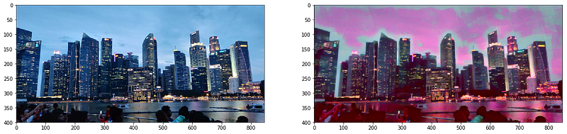
In the end, we can view the predicted results. I ran it for only a small number of iterations, but one can run up to 3000 iterations (if computation resources are no bar!).
def tensor_to_image(tensor):
    image = tensor.to("cpu").clone().detach()
    image = image.numpy().squeeze()
    image = image.transpose(1, 2, 0)
    image *= np.array((0.22, 0.22, 0.22))
                       + np.array((0.44, 0.44, 0.44))
    image = image.clip(0, 1)
    return image
fig, (ax1, ax2) = plt.subplots(1, 2, figsize=(20, 10))
ax1.imshow(tensor_to_image(img1))
ax2.imshow(tensor_to_image(target))
End Notes
There are plenty of other use cases where PyTorch can, and has been used. It has quickly become the darling of researchers around the globe. The majority of the open-source libraries and developments you’ll see happening nowadays have a PyTorch implementation available on GitHub.
In this article, I have illustrated what PyTorch is and how you can get started with implementing it in different use cases in deep learning. One should treat this guide as the starting point. The performance in every use case can be improved with more data, more fine-tuning of network parameters, and most importantly, applying creative skills while building network architectures. Thanks for reading and do leave your feedback in the comments section below.
References
- Official PyTorch Guide: https://pytorch.org/tutorials/
- Deep Learning with PyTorch: https://pytorch.org/tutorials/beginner/deep_learning_60min_blitz.html
- Faizan’s Article on AnalyticsVidhya: https://www.analyticsvidhya.com/blog/2018/02/pytorch-tutorial/
- Udacity Deep Learning using Pytorch: https://github.com/udacity/deep-learning-v2-pytorch
- Image Style Transfer Original Paper: https://www.cv-foundation.org/openaccess/content_cvpr_2016/papers/Gatys_Image_Style_Transfer_CVPR_2016_paper.pdf
Shivam5992 Bansal
27 Aug, 2021
Shivam Bansal is a data scientist with exhaustive experience in Natural Language Processing and Machine Learning in several domains. He is passionate about learning and always looks forward to solving challenging analytical problems.


Hey thanks for this Guide. Can you please share the performance benchmarks of keras vs tensorflow vs pytorch.
Hello Shivam Bassal i tried create code based your tutorial Use Case no 2 and i found error. could you share full code ? Thank you
For use case #2, Objects Image Classification I get as predicted labels numeric values instead of strings. Why is that?
In the NLP segment we are defining the model class and below piece is giving error: self.embedding = nn.Embedding(max_features, embedding_dim) Where are we defining max_features and embedding_dim? Request help on this.