Introduction
Us humans are supremely adept at glancing at any image and understanding what’s within it. In fact, it’s an almost imperceptible reaction from us. It takes us a fraction of a second to analyze.
It’s a completely different ball game for machines. There have been numerous attempts over the last couple of decades to make machines smarter at this task – and we might finally have cracked it, thanks to deep learning (and computer vision) techniques!
These deep learning algorithms are especially prevalent in our smartphone cameras. They analyze every pixel in a given image to detect objects, blur the background, and a whole host of tricks.
Most of these smartphones use multiple cameras to create that atmosphere. Google is in a league of its own, though. And I am delighted to be sharing an approach using their DeepLab V3+ model, which is present in Google Pixel phones, in this article!
Let’s build your first image segmentation model together!
This article requires a good understanding of Convolutional Neural Networks (CNNs). Head over to the below article to learn about CNNs (or get a quick refresher):
Table of contents
- Introduction
- Introduction to Image Segmentation
- Algorithms for Image Segmentation
- Getting Started with Google’s DeepLab
- Introduction to Atrous Convolutions
- Depthwise Separable Convolutions
- Depthwise Convolution
- Pointwise Convolution
- Understanding the DeepLab Model Architecture
- Training DeepLabV3+ on a Custom Dataset
- Conclusion
- Frequently Asked Questions
Introduction to Image Segmentation
Image segmentation is the task of partitioning an image into multiple segments. This makes it a whole lot easier to analyze the given image. And essentially, isn’t that what we are always striving for in computer vision? The below image perfectly illustrates the results of image segmentation:
Source:gfycat
This is quite similar to grouping pixels together on the basis of specific characteristic(s). Now these characteristics can often lead to different types of image segmentation, which we can divide into the following:
- Semantic Segmentation
- Instance Segmentation
Let’s take a moment to understand these concepts.
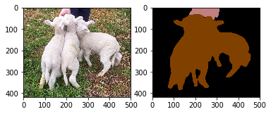
1. Semantic Segmentation
Check out the below image:
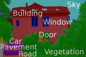
This is a classic example of semantic segmentation at work. Every pixel in the image belongs to one a particular class – car, building, window, etc. And all pixels belonging to a particular class have been assigned a single color. Awesome, right?
To formally put a definition to this concept,
Semantic segmentation is the task of assigning a class to every pixel in a given image.
Note here that this is significantly different from classification. Classification assigns a single class to the whole image whereas semantic segmentation classifies every pixel of the image to one of the classes.
Two popular applications of semantic segmentation include:
- Self-driving vehicles: These rely heavily on such segmented images to navigate through routes
- Portrait mode on Google’s Pixel phone: Here, instead of multiple classes, we need to classify every pixel as either belonging to the foreground or the background and then blurring the background part of the image
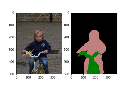
2. Instance Segmentation
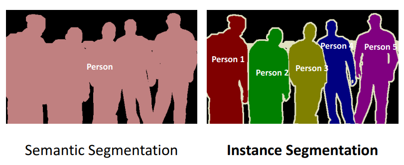
I love the above image! It neatly showcases how instance segmentation differs from semantic segmentation. Take a second to analyze it before reading further.
Different instances of the same class are segmented individually in instance segmentation. In other words, the segments are instance-aware. We can see in the above image that different instances of the same class (person) have been given different labels.
Algorithms for Image Segmentation
Image segmentation is a long standing computer Vision problem. Quite a few algorithms have been designed to solve this task, such as the Watershed algorithm, Image thresholding , K-means clustering, Graph partitioning methods, etc.
Many deep learning architectures (like fully connected networks for image segmentation) have also been proposed, but Google’s DeepLab model has given the best results till date. That’s why we’ll focus on using DeepLab in this article.
Getting Started with Google’s DeepLab
DeepLab is a state-of-the-art semantic segmentation model designed and open-sourced by Google back in 2016. Multiple improvements have been made to the model since then, including DeepLab V2 , DeepLab V3 and the latest DeepLab V3+.
We will understand the architecture behind DeepLab V3+ in this section and learn how to use it on our custom dataset.
The DeepLab model is broadly composed of two steps:
- Encoding phase: The aim of this phase is to extract essential information from the image. This is done using a pre trained Convoutional Neural Network , now you might be wondering why a CNN?
If you have previously worked with a CNN for image classification then you might know that convolutional layers look for different features in an image and pass this information to subsequent layers , now for segmentation task what comprises the essential information, its the objects present in the image and their location and since CNN are excellent at performing classification, they can easily find out the objects present. - Decoding phase: The information extracted in encoding phase is used here to reconstruct output of appropriate dimensions
What kind of techniques are used in both these phases? Let’s find out!
Understanding the Techniques used in the Encoding and Decoding Phases
The DeepLab architecture is based on combining two popular neural network architectures:
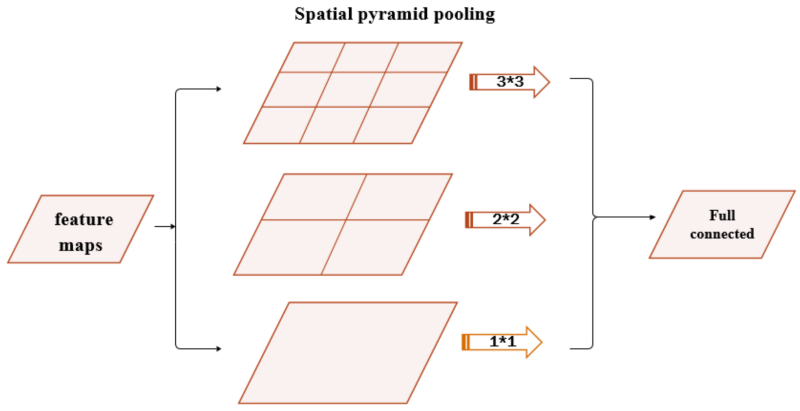
We need to make sure our model is robust to changes in the size of objects when working with CNNs. This is because if our model was trained using only images of small objects, then it might not perform well with scaled versions of the input images.
This problem can be resolved by using spatial pyramid pooling networks. These use multiple scaled versions of the input for training and hence capture multi-scale information.
Spatial pyramid pooling networks are able to encode multi-scale contextual information. This is done by probing the incoming features or pooling operations at multiple rates and with an effective field of view.
Spatial pyramid pooling networks generally use parallel versions of the same underlying network to train on inputs at different scales and combine the features at a later step.
Not everything present in the input will be useful for our model. We would want to extract only the crucial features that can be used to represent most of the information. That’s just a good rule of thumb to follow in general.
This is where the Encoder-Decoder networks perform well. They learn to transform the input into a dense form that can be used to represent all the input information (even reconstruct the input).
Introduction to Atrous Convolutions
Spatial pyramid pooling uses multiple instances of the same architecture. This leads to an increase in the computational complexity and the memory requirements of training. Not all of us have GPUs running freely so how do we go about mitigating this?
As usual, Google has the answer.
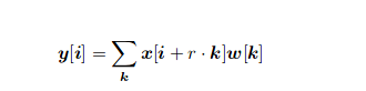
DeepLab has introduced the concept of atrous convolutions, a generalized form of the convolution operation. Atrous convolutions require a parameter called rate which is used to explicitly control the effective field of view of the convolution. The generalized form of atrous convolutions is given as:
The normal convolution is a special case of atrous convolutions with r = 1.
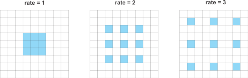
Hence, atrous convolutions can capture information from a larger effective field of view while using the same number of parameters and computational complexity.
DeepLab uses atrous convolution with rates 6, 12 and 18.
The name Atrous Spatial Pyramid Pooling (ASPP) was born thanks to DeepLab using Spatial Pyramid Pooling with atrous convolutions. Here, ASPP uses 4 parallel operations, i.e. 1 x 1 convolution and 3 x 3 atrous convolution with rates [6, 12, 18]. It also adds image level features with Global Average Pooling. Bilinear upsampling is used to scale the features to the correct dimensions.
Depthwise Separable Convolutions
Depthwise convolutions is a technique for performing convolutions with less number of computations than a standard convolution operation. This involves breaking down the convolution operation into two steps:
- Depthwise convolution
- Pointwise convolution
Let’s understand this using an example.
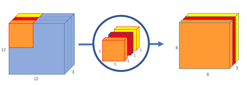
Suppose we have an image of size 12 x 12 composed of 3 channels. So, the shape of the input will be 12 x 12 x 3. We want to apply a convolution of 5 x 5 on this input.
Since we have 3 kernels of 5 x 5 for each input channel, applying convolution with these kernels gives an output shape of 8 x 8 x 1. We need to use more kernels and stack the outputs together in order to increase the number of output channels.
I’ll illustrate these two concepts using diagrams to give you an intuitive understanding of what we’re talking about.
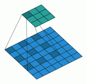
Depthwise Convolution
In this first step, we apply a convolution with a single kernel of shape 5 x 5 x 1, giving us an output of size 8 x 8 x 3:
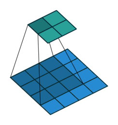
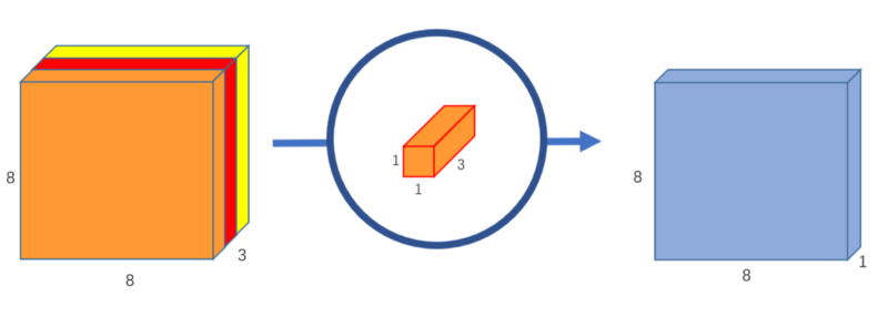
Pointwise Convolution
Now, we want to increase the number of channels. We’ll use 1 x 1 kernels with a depth matching the depth of the input image (3 in our case). This 1 x 1 x 3 convolution gives an output of shape 8 x 8 x 1. We can use as many 1 x 1 x 3 convolutions as required to increase the number of channels:
Let’s say we want to increase the number of channels to 256. What should we do? I want you to think about this before you see the solution.
We can use 256 1 x 1 x 3 over the input of 8 x 8 x 3 and get an output shape of 8 x 8 x 256.
Understanding the DeepLab Model Architecture
DeepLab V3 uses ImageNet’s pretrained Resnet-101 with atrous convolutions as its main feature extractor. In the modified ResNet model, the last ResNet block uses atrous convolutions with different dilation rates. It uses Atrous Spatial Pyramid Pooling and bilinear upsampling for the decoder module on top of the modified ResNet block.
DeepLab V3+ uses Aligned Xception as its main feature extractor, with the following modifications:
- All max pooling operations are replaced by depthwise separable convolution with striding
- Extra batch normalization and ReLU activation are added after each 3 x 3 depthwise convolution
- Depth of the model is increased without changing the entry flow network structure
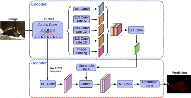
DeepLab V3+ Decoder
The encoder is based on an output stride (ratio of the original image size to the size of the final encoded features) of 16. Instead of using bilinear upsampling with a factor of 16, the encoded features are first upsampled with a factor of 4 and concatenated with corresponding low level features from the encoder module having the same spatial dimensions.
Before concatenating, 1 x 1 convolutions are applied on the low level features to reduce the number of channels. After concatenation, a few 3 x 3 convolutions are applied and the features are upsampled by a factor of 4. This gives the output of the same size as that of the input image.
Training DeepLabV3+ on a Custom Dataset
Let’s get our hands dirty with coding! First, clone Google research’s Github repo to download all the code to your local machine.
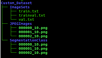
Preparing the dataset: For training the DeepLab model on our custom dataset, we need to convert the data to the TFRecord format. Move your dataset to model/research/deeplab/datasets. Our dataset directory should have the following structure:
TFRecord is TensorFlow’s custom binary data storage format. It makes it easier to work with huge datasets because binary data occupies much less space and can be read very efficiently.
The TFRecords format comes in very handy when working with datasets that are too large to be stored in the memory. Now only the data that’s required at the time is read from the disk. Sounds like a win-win!
- The JPEGImages folder contains the original images
- SegmentationClass folder contains the images with class labels as pixel values (it expects an image with a single channel where the value of every pixel is the classID)
- train.txt and val.txt contain the names of the images to be used for training and validation respectively
- trainval.txt contains names of all the images
Now, run the build_voc2012_data.py with the values of flags changed according to our directory structure. This converts your data to TFRecord format and saves it to the location pointed by ‘ — output_dir’.
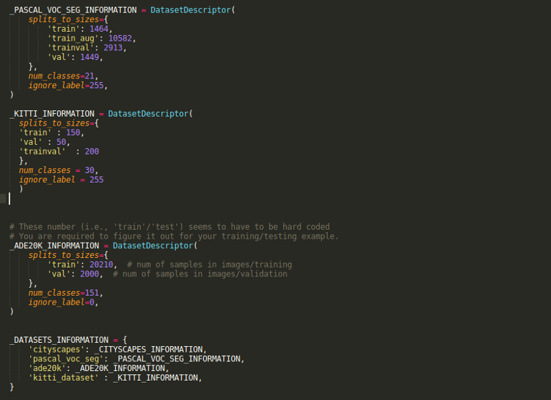
Open segmentation_dataset.py and add a DatasetDescriptor corresponding to your custom dataset. For example, we used the Pascal dataset with 1464 images for training and 1449 images for validation.
And now it’s time train our own image segmentation model!
Training our Image Segmentation Model
We need to run the train.py file present in the models/research/deeplab/ folder. Change the Flags according to your requirements.
# From tensorflow/models/research/
python deeplab/train.py \
   --logtostderr \
   --training_number_of_steps=90000 \
   --train_split="train" \
   --model_variant="xception_65" \
   --atrous_rates=6 \
   --atrous_rates=12 \
   --atrous_rates=18 \
   --output_stride=16 \
   --decoder_output_stride=4 \
   --train_crop_size=769 \
   --train_crop_size=769 \
   --train_batch_size=1 \
   --dataset="cityscapes" \
   --tf_initial_checkpoint=${PATH_TO_INITIAL_CHECKPOINT} \
This will train the model on your dataset and save the checkpoint files to train_logdir.
Evaluting our Image Segmentation Model
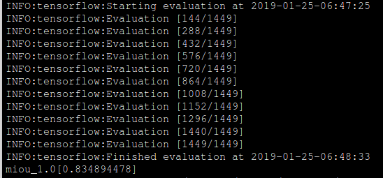
Now that we have the checkpoint files for our trained model, we can use them to evaluate its performance. Run the eval.py script with the changed FLAGs. This will evaluate the model on the images mentioned in the val.txt file.
python "${WORK_DIR}"/eval.py \
--logtostderr \
--eval_split="val" \
--model_variant="xception_65" \
--atrous_rates=6 \
--atrous_rates=12 \
--atrous_rates=18 \
--output_stride=16 \
--decoder_output_stride=4 \
--eval_crop_size=513 \
--eval_crop_size=513 \
--checkpoint_dir="${TRAIN_LOGDIR}" \
--eval_logdir="${EVAL_LOGDIR}" \
--dataset_dir="${PASCAL_DATASET}" \
--max_number_of_evaluations=1
We ran the training phase for 1000 steps and got meanIntersectionOverUnion of 0.834894478.
Remember that the the model_variant for both training and evaluation must be same.
Similarly, run vis.py with respective FLAGs for visualizing our results:
python "${WORK_DIR}"/vis.py \
--logtostderr \
--vis_split="val" \
--model_variant="xception_65" \
--atrous_rates=6 \
--atrous_rates=12 \
--atrous_rates=18 \
--output_stride=16 \
--decoder_output_stride=4 \
--vis_crop_size=513 \
--vis_crop_size=513 \
--checkpoint_dir="${TRAIN_LOGDIR}" \
--vis_logdir="${VIS_LOGDIR}" \
--dataset_dir="${PASCAL_DATASET}" \
--max_number_of_iterations=1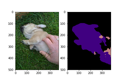
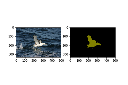
Let’s see some results from our trained model.
Looking good! Congratulations on training and running your first image segmentation model.
Conclusion
That was quite a lot of learning to digest! Once you’ve familiarized yourself with these concepts, try using it for your custom dataset (Kitti is a good choice because of its small size) and find out more cool practical use cases.
I strongly encourage you to check out the DeepLab paper and the Google AI blog post regarding this release:
Frequently Asked Questions
Q1.What is the difference between image classification and semantic segmentation?
Image Classification: Classifies the entire image into a single category or label, providing a high-level understanding of its content.
Semantic Segmentation: Identifies and classifies each pixel in an image, creating a detailed, pixel-level understanding and outlining the boundaries of different objects.
Q2. Which model is best for semantic segmentation?
The best model choice depends on the specific use case and requirements. Some popular semantic segmentation models include U-Net, FCN (Fully Convolutional Network), DeepLab, and PSPNet. The selection often considers factors like accuracy, speed, and resource efficiency.
Q3.What is the most popular semantic segmentation?
DeepLab is really popular. It’s good at catching small details in pictures. But remember, popularity can change, and there might be new models now.
I look forward to sharing your feedback, suggestions, and experience using DeepLab. You can connect with me in the comments section below.
Saurabh Pal
12 Dec, 2023
A Data Science enthusiast and Software Engineer by training, Saurabh aims to work at the intersection of both fields.


Hey,I'm trying to train my own dataset just like your tutorial (2 CLASS include backgroud) but i get black output The label image was a PNG format image with 2 color(0 for backround and 1 for foreground) SEG_INFORMATION = DatasetDescriptor( splits_to_sizes={ 'train': 300, # number of file in the train folder 'trainval': 30, 'val': 20, }, num_classes=2, # number of classes in your dataset ignore_label=255, # white edges that will be ignored to be class
In DatasetDesriptor, the value of trainval should be the sum of train and val i.e. 320 in your case, trainval represents all the images that are used for training and validation. Let me know if it solves your issue.
Great article! I am trying to train on my own dataset of size 299x299. I am able to produce the predicted masks, but they are all black. What am I supposed to put for the training and val_crop_size? I am confused. Thanks!
Thanks Joe, the val_crop_size is used in the image augmentation step. If you are not sure then you can use the model defaults and it should work fine. Larger values of val_crop_size might need more system memory.
Hello, the DeepLabV3+ source code on github has updated recently, and I try to use the latest code with my dataset about classroom. However, when i try to run eval.py, it stoped after print 'Starting evaluation..',and when i run vis.py, the output images are black. Can you help me to solve my problems?
Awesome article, I was curious what is the best was to create the images for the SegmentationClass folder? I am curious what examples of these images would look like?
Thanks for the great article..!! I'm stuck at converting into TFrecord... "NotFoundError: NewRandomAccessFile failed to Create/Open: C:\Users\Kishore\Downloads\models-master\models-master\research\deeplab\testing\pascal_voc_seg\VOCdevkit\VOC2012\JPEGImages\2008_000006.png : The system cannot find the file specified. ; No such file or directory" This is the error I'm getting.. Could you resolve it.. Thanks in advance...
Thank you for this great tutorial, it looks really great! But unfortunately I run into problems, and searching the net doesn't give any clues :( The Github DL3+ project has changed in the meantime (it seems a lot different from the 2018 version), and the file segmentation_dataset.py has been moved to 'deprecated'. And Github doesn't seem to have an archive (and archive.org didn't backup the project very well), so I can't simply load the old version. I'm just starting to learn AI and Python (I have lots of C/C++ programming experience), and can't find how to make it work with my own dataset. I was able to create the TFRecords using your tutorial, but after that I'm stuck. Where can I define the dataset that DL3+ will use for training? Or do you have the original DL3+ code somewhere that works with your tutorial? Would really appreciate your help, I'm stuck for two weeks now... Thank you in advance! Best regards, Robert