Decoding the Black Box: An Important Introduction to Interpretable Machine Learning Models in Python
Overview
- Interpretable machine learning is a critical concept every data scientist should be aware of
- How can you build interpretable machine learning models? This article will provide a framework
- We will also code these interpretable machine learning models in Python
Introduction
Can you interpret a deep neural network? How about a random forest with 500 trees? Building a complex and dense machine learning model has the potential of reaching our desired accuracy, but does it make sense? Can you open up the black-box model and explain how it arrived at the final result?
These are critical questions we need to answer as data scientists. A wide variety of businesses are relying on machine learning to drive their strategy and spruce up their bottomline. Building a model that we can explain to our clients and stakeholders is key.

Can you imagine building a facial recognition software that misclassifies a person? Or a credit card fraud detection model that raises an alarm for a perfectly legal transaction? And then not being able to explain why that’s happening – not ideal.
So the question is – how do we build interpretable machine learning models? That’s what we will talk about in this article. We’ll first understand what interpretable machine learning is and why it’s important. Then we will understand a simple framework for interpretable ML and use that to build machine learning models.
This is a very important topic in machine learning so strap in for a thrilling learning journey!
Interpretable machine learning is part of the comprehensive ‘Applied Machine Learning’ course. The course provides you all the tools and techniques you need to solve business problems using machine learning. It is an end-to-end course for beginners as well as intermediate-level professionals!
Table of Contents
- What is Interpretable Machine Learning?
- Why do we Need Interpretable Machine Learning?
- When can we do Away with Interpretability?
- Framework for Interpretable Machine Learning
- Let’s Talk About Inherently Interpretable Models
- Model Agnostic Techniques for Interpretable Machine Learning
- LIME (Local Interpretable Model Agnostic Explanations)
- Python Implementation of Interpretable Machine Learning Techniques
What is Interpretable Machine Learning?
How do we build trust in machine learning models? That’s essentially what this boils down to.
Machine learning-powered applications have become an ever-increasing part of our lives, from image and facial recognition systems to conversational applications, autonomous machines, and personalized systems.
The sort of decisions and predictions being made by these machine learning-enabled systems are becoming much more profound, and in many cases, critical to life, death, and personal wellness. The need to trust these AI-based systems is paramount.
So, let’s first take a step back and ask the question: What involves a predictive modeling lifecycle?
- Defining the problem statement?
- Hypothesis generation?
- Data exploration?
- Preprocessing?
- Feature Engineering?
- Deploying the model?
All these steps are involved in almost all problems based on structured datasets. However, a key issue that arises especially as model complexity increases is interpretability. Let’s start with the formal definition:
Interpretation of a machine learning model is the process wherein we try to understand the predictions of a machine learning model.
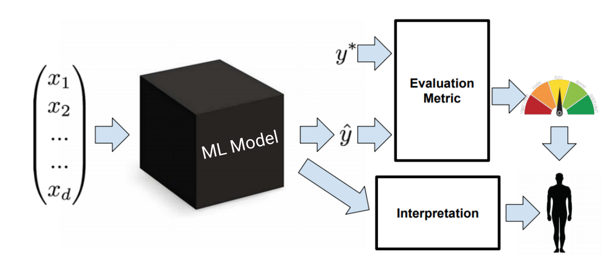
The involvement of humans in a predictive modeling lifecycle is at two important stages:
- One – where we monitor the evaluation metric and try different ideas of feature engineering, feature selection and algorithm selection to improve and build more robust models
- The second stage, which is the focus of this article, is to interpret the models using the predictions and parameters to understand why the classifier chose a particular class for example
Why do we Need Interpretable Machine Learning?
Before we jump into various kinds of techniques for interpreting machine learning models, let’s look at why this is important.
Fairness
Let’s take a simple example to understand this. Suppose we are trying to predict employees’ performance in a big company to expedite the appraisal process and identify the best employees.
We have data from the last 10 years about the performance reviews of employees. But what if that company tends to promote more men than women?

In this case, the model might learn the bias and predict that men tend to perform at a higher scale (and this bias has unfortunately happened in certain real-world scenarios). Now, if there is no way to interpret our model at this stage, the model might end up providing false insights at the cost of compromising on fairness.
Checking causality of features & Debugging models
Let’s consider another example. Consider that we are building a model for classifying wolves vs dogs. The data that is available is simply labeled images of dogs and wolves.
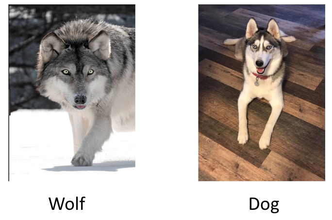
Now, what if we have wolves and dogs in entirely different backgrounds? This is entirely possible as wolves are mostly found in the wild (in snow, jungles, etc.) while dogs are in completely different backgrounds (households) generally.
We built an image classifier and got a really good performance on the validation set.
But on using one of the interpretability methods, we see that our model is actually ignoring the dog and wolf while using just the background pixels for doing the classification. This model might give a good performance on the validation set as they contain different backgrounds for the wolf and dog respectively.

Having an interpretable model, in this case, enables us to test the causality of the features, test its reliability and ultimately can help us to debug the model appropriately.
For example, we can try to alter our data by adding images of the animals in different backgrounds or simply crop the background out of the images to ensure that the right signal is picked up by our machine learning or deep learning model.
Regulations
Based on the latest regulations by the EU, GDPR’s article 12 allows individuals to enquire about algorithmic decisions. For example, in the banking and finance industry, questions such as the following can come up and have to be answered by these banks:
- Why was my loan rejected?
- Why did I get a low Credit Limit on my credit card? etc.

When can we do Away with Interpretability?
Not everything requires interpretability. It is also important to understand when we do not need to invest in building interpretable machine learning models.

- When interpretability does not impact the end customer. For example, a situation where we are looking to refine some internal processes. Say we want to classify the call recordings since a call resulted in a dissatisfied customer. We are good to go as long as we are getting a good performance and it is solving our purpose

- If the problem is well studied, we are confident about the results. For example, optical character recognition for which we can get a lot of training data and can rely on a good performance for the task at hand
Framework for Interpretable Machine Learning
Now that we have an intuition of what ML interpretability is and why it’s important, let’s look at the different ways to classify interpretability techniques:
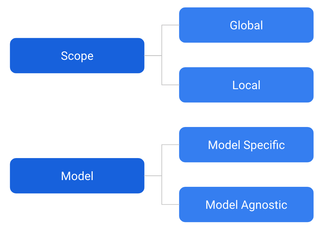
Overall we can think of interpretability under two structures:
Scope
Whether we are looking to interpret globally for all data points, the importance of each variable, or are we looking to explain a particular prediction which is local?
Model
The second way of looking at this is whether we are talking about a technique that works across all types of models (model agnostic) or is tailor-made for a particular class of algorithms (model specific).
Let’s Talk About Inherently Interpretable Models
Linear/Logistic
For linear models such as a linear and logistic regression, we can get the importance from the weights/coefficients of each feature.
Let’s revisit that quickly. Suppose we are trying to predict an employee’s salary using linear regression. The independent variables are experience in years and a previous rating out of 5.

For normalized data, W1 and W2 can essentially tell us whether the experience is more important towards salary or rating. Here, note that this is a model-specific technique that can be used for both global and local explanations.
Learn more about linear and logistic regression in the below articles:
Decision Trees
A decision tree is another algorithm that is very interpretable as we have access to all the splits for each feature:
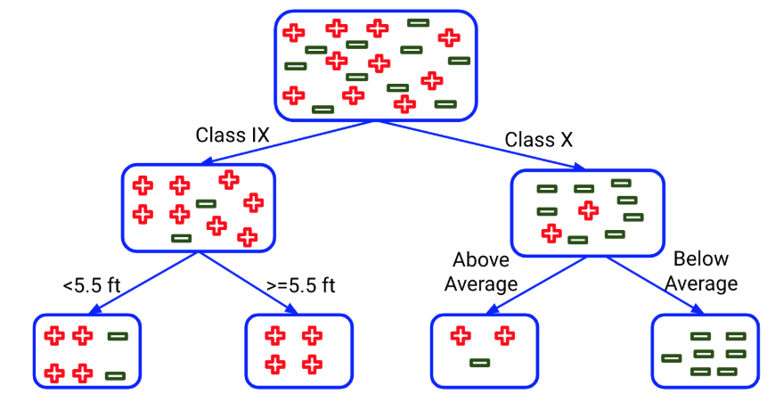
We can clearly see how the decisions are being taken starting from the root node to the leaf node. We just have to follow the rules on the basis of independent variables and list them down to explain each prediction. Again, this is a model-specific technique that can be used for local explanations.
What about global explanations?
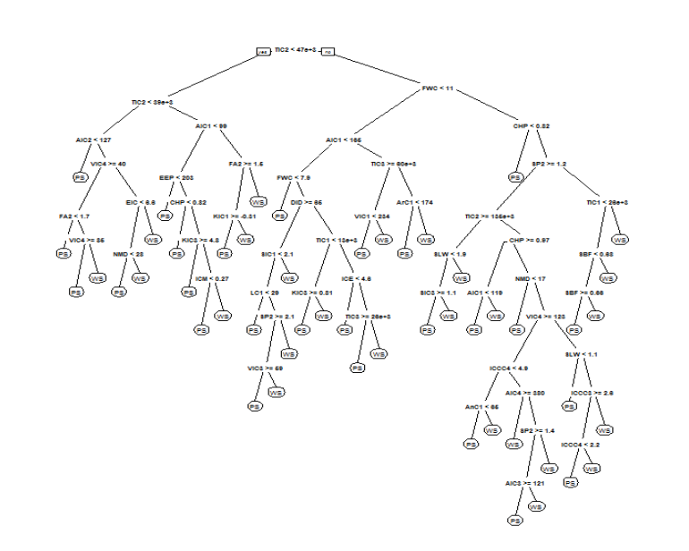
For a small decision tree, we can use the above diagram. However, if we have a lot of features and we are training a deep decision tree for, let’s say, a depth of 8 or 9, there will be too many decision rules to present effectively. In this case, we can use feature importance to interpret the importance of each feature at a global level.
Now, let’s learn how we can calculate feature importance for a decision tree.
Decision trees make splits to maximize the decrease in impurity. We can use this reduction to measure the contribution of each feature.
Let’s see how this works:
- Step 1: Go through all the splits in which the feature was used
- Step 2: Measure the reduction in criterion (Gini/information gain) compared to the parent node weighted by the number of samples. These weights are important as they help us incorporate the number of samples being segregated by the given feature as well into the equation. The formula is:
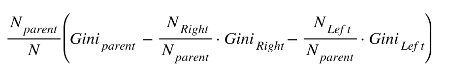
Here,
-
- N is the total number of observations
- N & Gini represents the number of samples & Gini impurity in the parent, left and right node
- Step 3: Take the sum for all splits for each feature and compare
Here, again, this is a model-specific technique that can be used for only global explanations. This is because we are looking at the overall importance and not at each prediction.
Learn more about decision trees in this superb tutorial.
An Example of Feature Importance
Now, let us try to understand this with an example. This will help you visualize what we’ve covered so far (and understand its importance).
Let’s say we have a decision tree with 4 samples and Gini impurity values as shown in the below figure. Each feature here appears only once so we can directly use the formula to calculate feature importance:
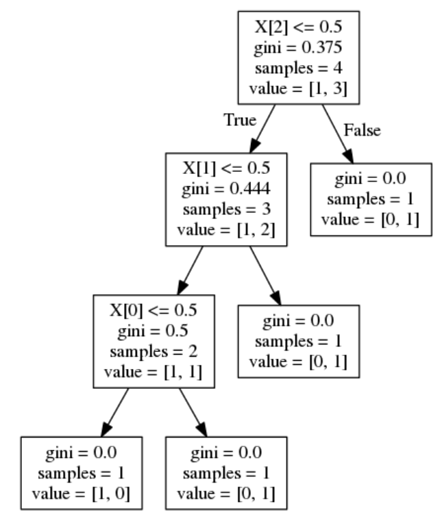
Since each feature is used once in our case, there is no need to calculate the sum.
- For X[2] :
- feature_importance = (4 / 4) * (0.375 – (0.75 * 0.444)) = 0.042
- For X[1] :
- feature_importance = (3 / 4) * (0.444 – (2/3 * 0.5)) = 0.083
- For X[0] :
- feature_importance = (2 / 4) * (0.5) = 0.25
Take a moment to pause here and calculate this on your own. You will have a much better grasp on the concept once you do it by yourself.
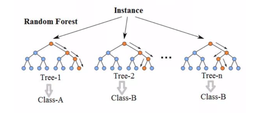
Tree Ensembles
Now, for tree ensembles such as random forest and Gradient Boosting Machines, we can use the same feature importance. But this time, we will take its average across all trees. Let us look at the steps involved:
- Go through each tree in the ensemble
- Find the feature importance by using the technique explained in the above section
- Take the average of all feature importance across all trees using this formula:

The popular sklearn library uses this technique to find feature importance for each feature.
Here are two intuitive guides to learn about Random Forest and Ensembling:
- Introduction to Random Forest – Simplified
- A Comprehensive Guide to Ensemble Learning (with Python codes)
Model Agnostic Techniques
So far, we have discussed model-specific techniques for linear and logistic regression, as well as decision trees. We also spoke about the feature importance methods that are used for ensemble methods. I’m sure you’re wondering – what about other models?
Now, we know that some models are hard to interpret, such as random forest and gradient boosting.
 We did use feature importance for these techniques. But it does not tell us whether a particular feature affects the target positively or negatively. And that is VERY important in certain cases.
Some machine learning models are even harder to interpret. For example, a deep neural network model can have millions of learned parameters and it essentially ends up being an extreme version of a black-box model.
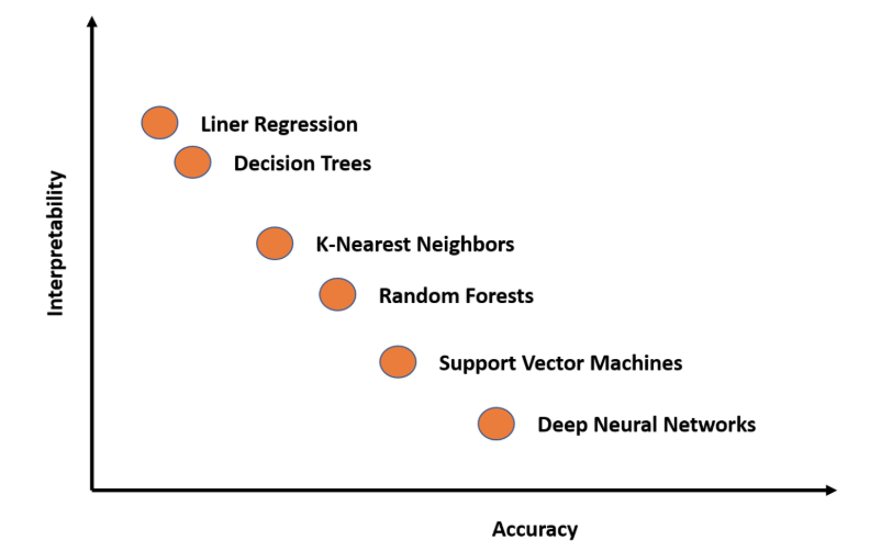
I really like this plot. As the complexity of the machine learning model increases, we get better performance but lose out on interpretability. You should keep this figure handy the next time you’re building your own model.
So how can we build interpretable machine learning models that don’t compromise on accuracy?
One idea is to use simpler models. That way you can ensure you have full confidence in the interpretability. However, complex models can provide much better performance. So is there a way we can have some level of interpretability for black-box models as well?
Yes! Model agnostic techniques allow us to build and use more complex models without losing all interpretability power.
Let’s take a high-level look at model-agnostic interpretability. We capture the world by collecting data, and abstract it further by learning to predict the data with a machine learning model. Interpretability is just another layer on top that helps humans understand the black box using a simpler, more interpretable model.
Global Surrogate Method
The first model agnostic method we will discuss here is the global surrogate method. A global surrogate model is an interpretable model that is trained to approximate the predictions of a black-box model.
We can draw conclusions about the black-box model by interpreting the surrogate model. So, we are basically solving machine learning interpretability by using more machine learning!
For example, we could interpret a random forest classifier using a simple decision tree to explain its predictions:
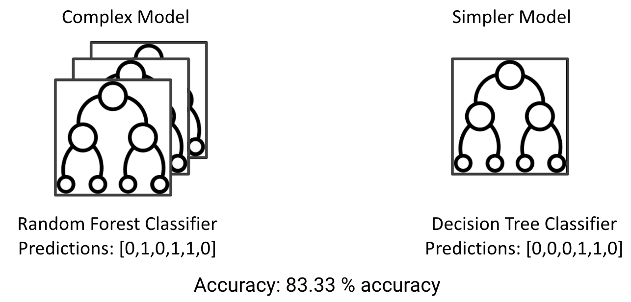
This is done by training a decision tree on the predictions of the black-box model (which is a random forest in our case). And once it provides good enough accuracy, we can use it to explain the random forest classifier.
Overall, we want an interpretable surrogate model that is trained to approximate the predictions of a black-box model and draw conclusions.
Here is a step-by-step breakdown to understand how a global surrogate model works:
- We get predictions from the black-box model
- Next, we select an interpretable model (Linear, decision tree, etc.)
- We train an interpretable model on the original dataset and use black box predictions as the target
- Measure the performance of the surrogate model
- Finally, we interpret the surrogate model to understand how the black-box model is making its decisions
LIME (Local Interpretable Model agnostic Explanations)
The global surrogate method is good for looking at an interpretable model that can explain predictions for a black-box approach. However, this will not work well if we want to understand how a single prediction was made for a given observation.
This is where we use the LIME technique which stands for local interpretable model agnostic explanations. LIME is based on the work presented in this paper. Let us understand how LIME works using an example.
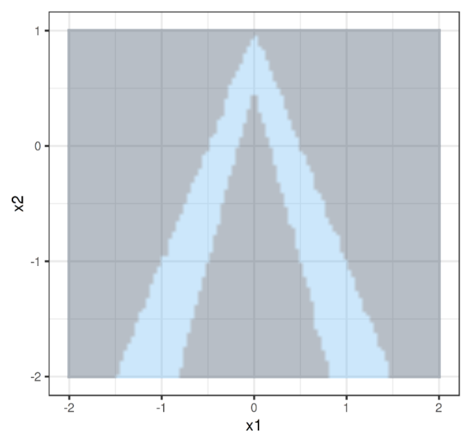
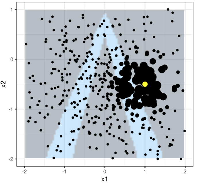
Suppose we are working on a binary classification problem. As we can see in the above image, we have a decision boundary for a black-box model with two features.
Let’s say we want to interpret the contributions of x1 and x2 for the observation in yellow (in the below image). We take the data sampled from a normal distribution to generate fake data around the observation:
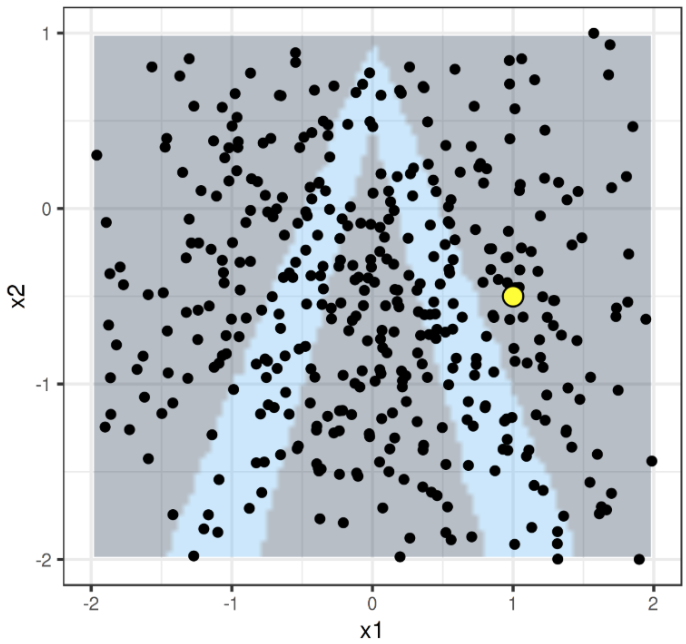
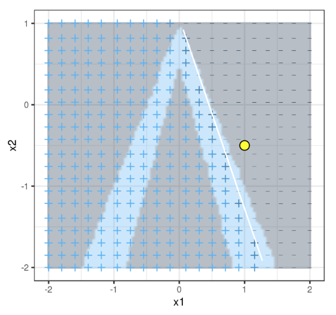
Next, we assign higher weights to the points that are closer to our observation:
We train an interpretable model over the fake data generated from the distribution. Now, we have a new local decision boundary for the locally learned model (in white) that can be used to understand the contributions of x1 and x2 towards the prediction of our observation:
Summarising all the steps:
- Select your instance of interest for which you want to have an explanation of its black box prediction
- Perturb your dataset and get the black box predictions for these new fake data points
- Weight the new samples according to their proximity to the instance of interest
- Train a weighted, interpretable model on the dataset with the variations
- Explain the prediction by interpreting the local model
Python Implementation of Interpretable Machine Learning Techniques
My favorite part of the article – building interpretable machine learning models in Python!
Here, we will work on the implementation of both the methods we covered above. We will use the big mart sales problem hosted on our Datahack Platform. The problem statement includes predicting sales for different items being sold at different outlets. You can download the dataset from the above link.
Note: You can go through this course to fully understand how to build models using this data. Our focus here is to focus on the interpretability part.
Building and Understanding Interpretable Machine Learning Models
Let us first look at how to do interpretability for inherently interpretable machine learning models.
Importing the Required Libraries
# importing the required libraries
import pandas as pd
import numpy as np
from sklearn.model_selection import train_test_split
from sklearn.metrics import mean_squared_error

from sklearn.linear_model import LinearRegression
from sklearn.tree import DecisionTreeRegressor
from sklearn.ensemble import RandomForestRegressor
from xgboost.sklearn import XGBRegressor
from sklearn.preprocessing import OneHotEncoder, LabelEncoder
from sklearn import tree

import matplotlib.pyplot as plt
%matplotlib inline
Reading Data
# reading the data
df = pd.read_csv('data.csv')
Missing Value Treatment
# imputing missing values in Item_Weight by median and Outlet_Size with mode
df['Item_Weight'].fillna(df['Item_Weight'].median(), inplace=True)
df['Outlet_Size'].fillna(df['Outlet_Size'].mode()[0], inplace=True)
Feature Engineering
# creating a broad category of type of Items
df['Item_Type_Combined'] = df['Item_Identifier'].apply(lambda df: df[0:2])
df['Item_Type_Combined'] = df['Item_Type_Combined'].map({'FD':'Food', 'NC':'Non-Consumable', 'DR':'Drinks'})

df['Item_Type_Combined'].value_counts()

# operating years of the store
df['Outlet_Years'] = 2013 - df['Outlet_Establishment_Year']

# modifying categories of Item_Fat_Content
df['Item_Fat_Content'] = df['Item_Fat_Content'].replace({'LF':'Low Fat', 'reg':'Regular', 'low fat':'Low Fat'})
df['Item_Fat_Content'].value_counts()
Data Preprocessing
# label encoding the ordinal variables
le = LabelEncoder()
df['Outlet'] = le.fit_transform(df['Outlet_Identifier'])
var_mod = ['Item_Fat_Content','Outlet_Location_Type','Outlet_Size','Item_Type_Combined','Outlet_Type','Outlet']
le = LabelEncoder()
for i in var_mod:
df[i] = le.fit_transform(df[i])

# one hot encoding the remaining categorical variables
df = pd.get_dummies(df, columns=['Item_Fat_Content','Outlet_Location_Type','Outlet_Size','Outlet_Type',
                              'Item_Type_Combined','Outlet'])
Train-Test Split
# dropping the ID variables and variables that have been used to extract new variables
df.drop(['Item_Type','Outlet_Establishment_Year', 'Item_Identifier', 'Outlet_Identifier'],axis=1,inplace=True)

# separating the dependent and independent variables
X = df.drop('Item_Outlet_Sales',1)
y = df['Item_Outlet_Sales']

# creating the training and validation set
X_train, X_test, y_train, y_test = train_test_split(X, y, test_size=.25, random_state=42)
Training a Decision Tree Model
dt = DecisionTreeRegressor(max_depth = 5, random_state=10)

# fitting the decision tree model on the training set
dt.fit(X_train, y_train)
Use the Graphviz library to visualize the decision tree
# Visualising the decision tree
decision_tree = tree.export_graphviz(dt, out_file='tree.dot', feature_names=X_train.columns, filled=True, max_depth=2)

# converting the dot image to png format
!dot -Tpng tree.dot -o tree.png

#plotting the decision tree
image = plt.imread('tree.png')
plt.figure(figsize=(25,25))
plt.imshow(image)
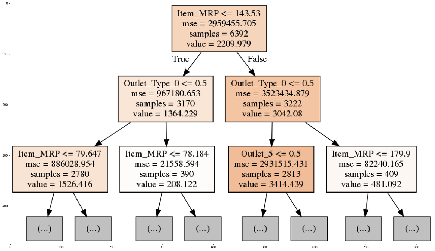
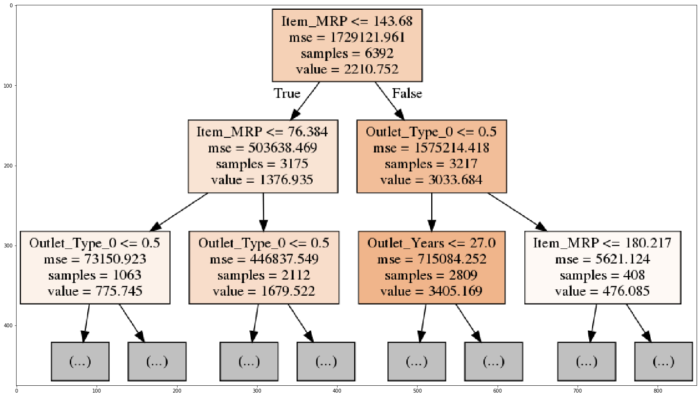
This visualization of our decision tree clearly displays the rules it is using to make a prediction. Here, Item_MRP & Outlet_Type are the first features that are affecting the sales of various items at each outlet. If you want to look at the complete decision tree, you can easily do that by changing the max_depth parameter using the export_graphviz function.
Feature Importance
Now, we will have a look at the feature importance for each feature in case of a random forest.
# creating the Random Forest Regressor model
rf = RandomForestRegressor(n_estimators=200, max_depth=5, min_samples_leaf=100,n_jobs=-1)

# feature importance of the random forest model
feature_importance = pd.DataFrame()
feature_importance['variable'] = X_train.columns
feature_importance['importance'] = rf.feature_importances_

# feature_importance values in descending order
feature_importance.sort_values(by='importance', ascending=False).head(10)
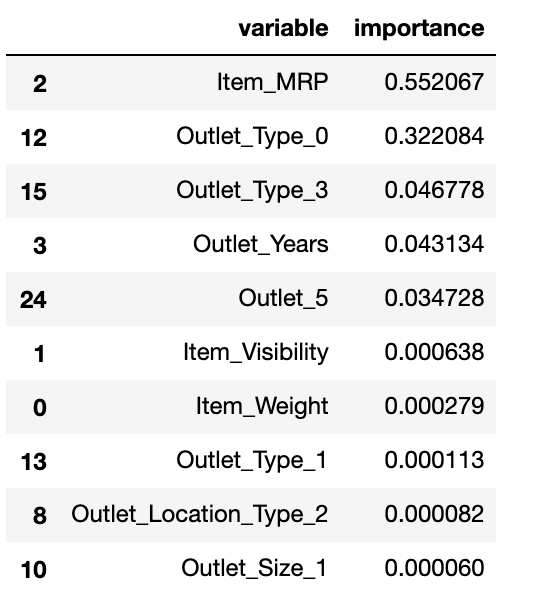
The random forest model gives a similar interpretation. Item_MRP still remains the most important feature (exactly as the decision tree model above). Relative importance also helps us compare each feature. For example, Outlet_Type_0 is a much more important feature than other outlet types.
Exercise
As an exercise try calculating the feature importance for the decision tree we fit earlier and compare:
Global Surrogate
Next, we will create a surrogate decision tree model for this random forest model and see what we get.
# saving the predictions of Random Forest as new target
new_target = rf.predict(X_train)

# defining the interpretable decision tree model
dt_model = DecisionTreeRegressor(max_depth=5, random_state=10)

# fitting the surrogate decision tree model using the training set and new target
dt_model.fit(X_train,new_target)
This decision tree performs well on the new target and can be used as a surrogate model to explain the predictions of a random forest model. Similarly, we can use it for any other complex model. Just make sure your decision tree fits well, otherwise, you might get wrong interpretations (a nightmare!).
Implementing LIME in Python to generate local interpretations of black-box models
We can implement the LIME technique in both R & Python using the LIME package. Let’s jump into implementation for the same to check the local interpretation of a given prediction using LIME:
# installing lime library
!pip install lime

# import Explainer function from lime_tabular module of lime library
from lime.lime_tabular import LimeTabularExplainer

# training the random forest model
rf_model = RandomForestRegressor(n_estimators=200,max_depth=5, min_samples_leaf=100,n_jobs=-1, random_state=10)
rf_model.fit(X_train, y_train)

# creating the explainer function
explainer = LimeTabularExplainer(X_train.values, mode="regression", feature_names=X_train.columns)

# storing a new observation
i = 6
X_observation = X_test.iloc[[i], :]

* RF prediction: {rf_model.predict(X_observation)[0]}
![]()
Generate Explanations using LIME
# explanation using the random forest model
explanation = explainer.explain_instance(X_observation.values[0], rf_model.predict)
explanation.show_in_notebook(show_table=True, show_all=False)
print(explanation.score)
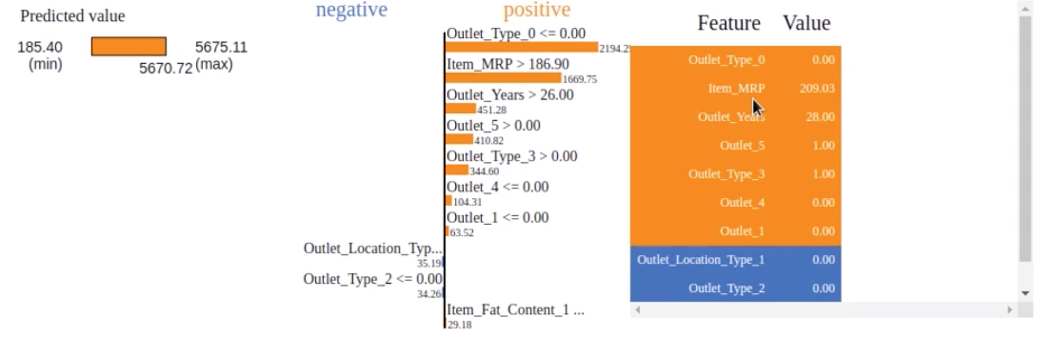
The predicted value for sales is 185.40. Each feature’s contribution to this prediction is shown in the right bar plot. Orange signifies the positive impact and blue signifies the negative impact of that feature on the target. For example, Item_MRP has a positive impact on sales.
Exercise 2
Using the coding window below, try applying LIME to more complex models such as Xgboost & LightGBM. The code for preprocessing and model building is already inserted here:
For more details on LIME and its implementation, you can go through this article.
End Notes
LIME is a powerful technique but has its disadvantages as it relies on locally generated fake data and uses simple linear models to explain predictions. However, it can be used for text and image data as well.
As I mentioned earlier, interpretable machine learning is part of our utterly comprehensive end-to-end course:
Make sure you check it out. And if you have any questions or feedback regarding this article, let me know in the comments section below.
IIT Bombay Graduate with a Masters and Bachelors in Electrical Engineering. I have previously worked as a lead decision scientist for Indian National Congress deploying statistical models (Segmentation, K-Nearest Neighbours) to help party leadership/Team make data-driven decisions. My interest lies in putting data in heart of business for data-driven decision making.


Can we calculate lime/shap values for sarima model with exogenous variables?