Feature Engineering for Images: A Valuable Introduction to the HOG Feature Descriptor
Introduction
Feature engineering is a game-changer in the world of machine learning algorithms. It’s actually one of my favorite aspects of being a data scientist! This is where we get to experiment the most – to engineer new features from existing ones and improve our model’s performance. You would even have used various feature engineering techniques on structured data. Can we extend this technique to unstructured data, such as images? It’s an intriguing riddle for computer vision enthusiasts and one we will solve in this article. In this article, we will introduce you to a popular feature extraction technique for images – Histogram of Oriented Gradients, or HOG feature extraction. We will understand what is the HOG feature descriptor, how it works (the complete math behind the algorithm), and finally, implement it in Python.
Overview
- Learn the inner workings and math behind the HOG feature descriptor
- The HOG feature descriptor is used in computer vision popularly for object detection
- A valuable feature engineering guide for all computer vision enthusiasts
Table of contents
- What is a Feature Descriptor?
- What is Histogram of Oriented Gradients?
- Introduction to the HOG Feature Descriptor
- Process of Calculating the Histogram of Oriented Gradients (HOG)
- Different Methods to Create Histograms using Gradients and Orientation
- Implementing HOG Feature Descriptor in Python
- Frequently Asked Questions
What is a Feature Descriptor?
You might have had this question since you read the heading. So let’s clear that up first before we jump into the HOG part of the article.
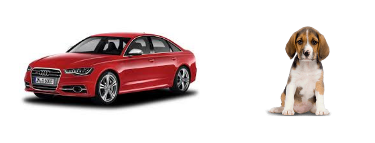
Take a look at the two images shown below. Can you differentiate between the objects in the image?
We can clearly see that the right image here has a dog and the left image has a car. Now, let me make this task slightly more complicated – identify the objects shown in the image below:
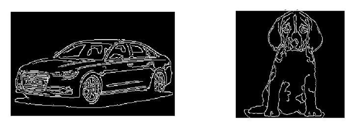
Still easy, right? Can you guess what was the difference between the first and the second case? The first pair of images had a lot of information, like the shape of the object, its color, the edges, background, etc.
On the other hand, the second pair had much less information (only the shape and the edges) but it was still enough to differentiate the two images.
Do you see where I am going with this? We were easily able to differentiate the objects in the second case because it had the necessary information we would need to identify the object. And that is exactly what a feature descriptor does:
It is a simplified representation of the image that contains only the most important information about the image.
There are a number of feature descriptors out there. Here are a few of the most popular ones:
- HOG: Histogram of Oriented Gradients
- SIFT: Scale Invariant Feature Transform
- SURF: Speeded-Up Robust Feature
In this article, we are going to focus on the HOG feature descriptor and how it works. Let’s get started!
What is Histogram of Oriented Gradients?
The Histogram of Oriented Gradients (HOG) is a popular feature descriptor technique in computer vision and image processing. It analyzes the distribution of edge orientations within an object to describe its shape and appearance. The HOG method involves computing the gradient magnitude and orientation for each pixel in an image and then dividing the image into small cells.
Introduction to the HOG Feature Descriptor
HOG, or Histogram of Oriented Gradients, is a feature descriptor that is often used to extract features from image data. It is widely used in computer vision tasks for object detection.
Let’s look at some important aspects of HOG that makes it different from other feature descriptors:
- The HOG descriptor focuses on the structure or the shape of an object. Now you might ask, how is this different from the edge features we extract for images? In the case of edge features, we only identify if the pixel is an edge or not. HOG is able to provide the edge direction as well. This is done by extracting the gradient and orientation (or you can say magnitude and direction) of the edges
- Additionally, these orientations are calculated in ‘localized’ portions. This means that the complete image is broken down into smaller regions and for each region, the gradients and orientation are calculated. We will discuss this in much more detail in the upcoming sections
- Finally the HOG would generate a Histogram for each of these regions separately. The histograms are created using the gradients and orientations of the pixel values, hence the name ‘Histogram of Oriented Gradients’
To put a formal definition to this:
The HOG feature descriptor counts the occurrences of gradient orientation in localized portions of an image.
Implementing HOG using tools like OpenCV is extremely simple. It’s just a few lines of code since we have a predefined function called hog in the skimage.feature library. Our focus in this article, however, is on how these features are actually calculated.
Process of Calculating the Histogram of Oriented Gradients (HOG)
We should now have a basic idea of what a HOG feature descriptor is. It’s time to delve into the core idea behind this article. Let’s discuss the step-by-step process to calculate HOG.
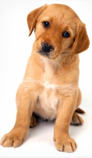
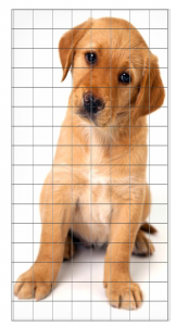
Consider the below image of size (180 x 280). Let us take a detailed look at how the HOG features will be created for this image:
Step 1: Preprocess the Data (64 x 128)
This is a step most of you will be pretty familiar with. Preprocessing data is a crucial step in any machine learning project and that’s no different when working with images.
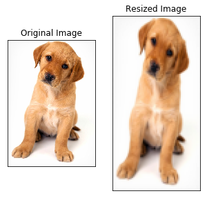
We need to preprocess the image and bring down the width to height ratio to 1:2. The image size should preferably be 64 x 128. This is because we will be dividing the image into 8*8 and 16*16 patches to extract the features. Having the specified size (64 x 128) will make all our calculations pretty simple. In fact, this is the exact value used in the original paper.
Coming back to the example we have, let us take the size 64 x 128 to be the standard image size for now. Here is the resized image:
Step 2: Calculating Gradients (direction x and y)
The next step is to calculate the gradient for every pixel in the image. Gradients are the small change in the x and y directions. Here, I am going to take a small patch from the image and calculate the gradients on that:
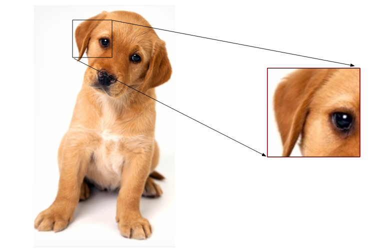
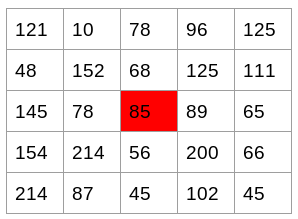
We will get the pixel values for this patch. Let’s say we generate the below pixel matrix for the given patch (the matrix shown here is merely used as an example and these are not the original pixel values for the given patch):
Source: Applied Machine Learning Course
I have highlighted the pixel value 85. Now, to determine the gradient (or change) in the x-direction, we need to subtract the value on the left from the pixel value on the right. Similarly, to calculate the gradient in the y-direction, we will subtract the pixel value below from the pixel value above the selected pixel.
Hence the resultant gradients in the x and y direction for this pixel are:
- Change in X direction(Gx) = 89 – 78 = 11
- Change in Y direction(Gy) = 68 – 56 = 8
This process will give us two new matrices – one storing gradients in the x-direction and the other storing gradients in the y direction. This is similar to using a Sobel Kernel of size 1. The magnitude would be higher when there is a sharp change in intensity, such as around the edges.
We have calculated the gradients in both x and y direction separately. The same process is repeated for all the pixels in the image. The next step would be to find the magnitude and orientation using these values.
Step 3: Calculate the Magnitude and Orientation
Using the gradients we calculated in the last step, we will now determine the magnitude and direction for each pixel value. For this step, we will be using the Pythagoras theorem (yes, the same one which you studied back in school!).
Take a look at the image below:
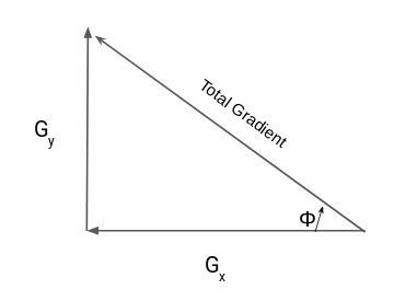
The gradients are basically the base and perpendicular here. So, for the previous example, we had Gx and Gy as 11 and 8. Let’s apply the Pythagoras theorem to calculate the total gradient magnitude:
Total Gradient Magnitude = √[(Gx)2+(Gy)2]
Total Gradient Magnitude = √[(11)2+(8)2] = 13.6
Next, calculate the orientation (or direction) for the same pixel. We know that we can write the tan for the angles:
tan(Φ) = Gy / Gx
Hence, the value of the angle would be:
Φ = atan(Gy / Gx)
The orientation comes out to be 36 when we plug in the values. So now, for every pixel value, we have the total gradient (magnitude) and the orientation (direction). We need to generate the histogram using these gradients and orientations.
But hang on – we need to take a small break before we jump into how histograms are created in the HOG feature descriptor. Consider this a small step in the overall process. And we’ll start this by discussing some simple methods of creating Histograms using the two values that we have – gradients and orientation.
Different Methods to Create Histograms using Gradients and Orientation
A histogram is a plot that shows the frequency distribution of a set of continuous data. We have the variable (in the form of bins) on the x-axis and the frequency on the y-axis. Here, we are going to take the angle or orientation on the x-axis and the frequency on the y-axis.
Method 1:
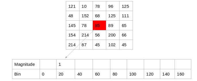
Let us start with the simplest way to generate histograms. We will take each pixel value, find the orientation of the pixel and update the frequency table.
Here is the process for the highlighted pixel (85). Since the orientation for this pixel is 36, we will add a number against angle value 36, denoting the frequency:

Source: Applied Machine Learning Course
The same process is repeated for all the pixel values, and we end up with a frequency table that denotes angles and the occurrence of these angles in the image. This frequency table can be used to generate a histogram with angle values on the x-axis and the frequency on the y-axis.
That’s one way to create a histogram. Note that here the bin value of the histogram is 1. Hence we get about 180 different buckets, each representing an orientation value. Another method is to create the histogram features for higher bin values.
Method 2:
This method is similar to the previous method, except that here we have a bin size of 20. So, the number of buckets we would get here is 9.
Again, for each pixel, we will check the orientation, and store the frequency of the orientation values in the form of a 9 x 1 matrix. Plotting this would give us the histogram:
Source: Applied Machine Learning Course
Method 3:
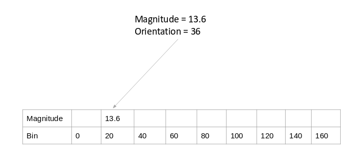
The above two methods use only the orientation values to generate histograms and do not take the gradient value into account. Here is another way in which we can generate the histogram – instead of using the frequency, we can use the gradient magnitude to fill the values in the matrix. Below is an example of this:
Source: Applied Machine Learning Course
You might have noticed that we are using the orientation value of 30, and updating the bin 20 only. Additionally, we should give some weight to the other bin as well.
Method 4:
Let’s make a small modification to the above method. Here, we will add the contribution of a pixel’s gradient to the bins on either side of the pixel gradient. Remember, the higher contribution should be to the bin value which is closer to the orientation.
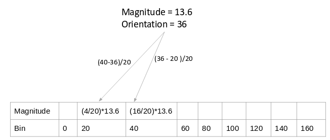
Source: Applied Machine Learning Course
This is exactly how histograms are created in the HOG feature descriptor.
Step 4: Calculate Histogram of Gradients in 8×8 cells (9×1)
The histograms created in the HOG feature descriptor are not generated for the whole image. Instead, the image is divided into 8×8 cells, and the histogram of oriented gradients is computed for each cell. Why do you think this happens?
By doing so, we get the features (or histogram) for the smaller patches which in turn represent the whole image. We can certainly change this value here from 8 x 8 to 16 x 16 or 32 x 32.
If we divide the image into 8×8 cells and generate the histograms, we will get a 9 x 1 matrix for each cell. This matrix is generated using method 4 that we discussed in the previous section.
Once we have generated the HOG for the 8×8 patches in the image, the next step is to normalize the histogram.
Step 5: Normalize gradients in 16×16 cell (36×1)
Before we understand how this is done, it’s important to understand why this is done in the first place.
Although we already have the HOG features created for the 8×8 cells of the image, the gradients of the image are sensitive to the overall lighting. This means that for a particular picture, some portion of the image would be very bright as compared to the other portions.
We cannot completely eliminate this from the image. But we can reduce this lighting variation by normalizing the gradients by taking 16×16 blocks. Here is an example that can explain how 16×16 blocks are created:
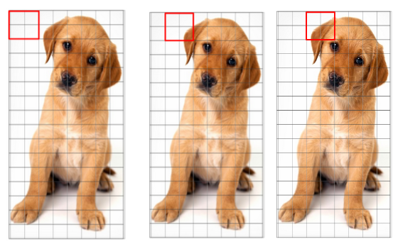
Here, we will be combining four 8×8 cells to create a 16×16 block. And we already know that each 8×8 cell has a 9×1 matrix for a histogram. So, we would have four 9×1 matrices or a single 36×1 matrix. To normalize this matrix, we will divide each of these values by the square root of the sum of squares of the values. Mathematically, for a given vector V:
V = [a1, a2, a3, ….a36]
We calculate the root of the sum of squares:
k = √(a1)2+ (a2)2+ (a3)2+ …. (a36)2
And divide all the values in the vector V with this value k:
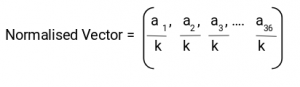
The resultant would be a normalized vector of size 36×1.
Step 6: Features for the complete image
We are now at the final step of generating HOG features for the image. So far, we have created features for 16×16 blocks of the image. Now, we will combine all these to get the features for the final image.
Can you guess what would be the total number of features that we will have for the given image? We would first need to find out how many such 16×16 blocks would we get for a single 64×128 image:
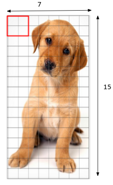
We would have 105 (7×15) blocks of 16×16. Each of these 105 blocks has a vector of 36×1 as features. Hence, the total features for the image would be 105 x 36×1 = 3780 features.
We will now generate HOG features for a single image and verify if we get the same number of features at the end.
Implementing HOG Feature Descriptor in Python
Time to fire up Python! This, I’m sure, is the most anticipated section of this article. So let’s get rolling.
We will see how we can generate HOG features on a single image, and if the same can be applied on a larger dataset. We will first load the required libraries and the image for which we are going to create the HOG features:
#importing required libraries
from skimage.io import imread, imshow
from skimage.transform import resize
from skimage.feature import hog
from skimage import exposure
import matplotlib.pyplot as plt
%matplotlib inline


#reading the image
img = imread('puppy.jpeg')
imshow(img)
print(img.shape)
view rawreading_image.py hosted with ❤ by GitHub
(663, 459, 3)
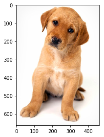
We can see that the shape of the image is 663 x 459. We will have to resize this image into 64 x 128. Note that we are using skimage which takes the input as height x width.
#resizing image
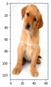
resized_img = resize(img, (128,64))
imshow(resized_img)
print(resized_img.shape)(128, 64, 3)
Here, I am going to use the hog function from skimage.features directly. So we don’t have to calculate the gradients, magnitude (total gradient) and orientation individually. The hog function would internally calculate it and return the feature matrix.
Also, if you set the parameter ‘visualize = True’, it will return an image of the HOG.
#creating hog features
fd, hog_image = hog(resized_img, orientations=9, pixels_per_cell=(8, 8),
                    cells_per_block=(2, 2), visualize=True, multichannel=True)
Before going ahead, let me give you a basic idea of what each of these hyperparameters represents. Alternatively, you can check the definitions from the official documentation here.
- The orientations are the number of buckets we want to create. Since I want to have a 9 x 1 matrix, I will set the orientations to 9
- pixels_per_cell defines the size of the cell for which we create the histograms. In the example we covered in this article, we used 8 x 8 cells and here I will set the same value. As mentioned previously, you can choose to change this value
- We have another hyperparameter cells_per_block which is the size of the block over which we normalize the histogram. Here, we mention the cells per blocks and not the number of pixels. So, instead of writing 16 x 16, we will use 2 x 2 here
The feature matrix from the function is stored in the variable fd, and the image is stored in hog_image. Let us check the shape of the feature matrix:
fd.shape(3780,)
As expected, we have 3,780 features for the image and this verifies the calculations we did in step 7 earlier. You can choose to change the values of the hyperparameters and that will give you a feature matrix of different sizes.
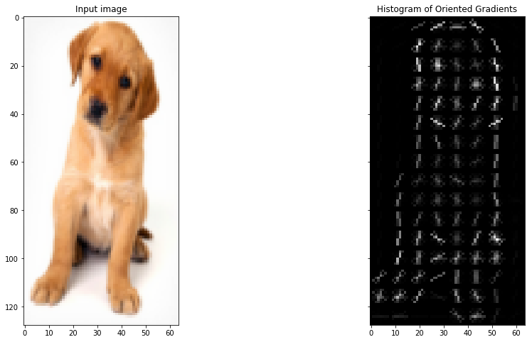
Let’s finally look at the HOG image:
fig, (ax1, ax2) = plt.subplots(1, 2, figsize=(16, 8), sharex=True, sharey=True)

ax1.imshow(resized_img, cmap=plt.cm.gray)
ax1.set_title('Input image')

# Rescale histogram for better display
hog_image_rescaled = exposure.rescale_intensity(hog_image, in_range=(0, 10))

ax2.imshow(hog_image_rescaled, cmap=plt.cm.gray)
ax2.set_title('Histogram of Oriented Gradients')

plt.show()
Conclusion
The idea behind this article was to give you an understanding of what is actually happening behind the HOG feature descriptor and how the features are calculated. The complete process is broken down into 7 simple steps. As a next step, we would encourage you to try using HOG features on a simple computer vision problem and see if the model performance improves. Do share your results in the comment section!
Frequently Asked Questions
A. A HOG (Histogram of Oriented Gradients) feature is a feature descriptor used in computer vision and image processing for object detection and recognition. Its feature descriptor represents an image’s gradient or edge orientation patterns as a histogram in machine learning models to recognize objects.
A. In image processing, HOG features refer to the image features extracted using the HOG algorithm. The HOG algorithm divides an image into small cells, computes each cell’s gradient orientation and magnitude, and then aggregates the gradient information into a histogram of oriented gradients. These histograms describe the image features and detect objects within an image.
A. In Python, the HOG feature descriptor can be extracted using the scikit-image library, which provides functions to compute HOG features from images. The HOG feature extraction process involves specifying the histogram computation’s cell size, block size, and number of orientations.
A. The size of HOG features depends on the parameters used in the feature extraction process, such as cell and block sizes. Generally, larger cell and block sizes will result in larger HOG features, while smaller sizes will result in smaller features. The size of the HOG features can impact the performance of machine learning models. Choosing appropriate parameters for the feature extraction process is important in object detection and recognition tasks.
An avid reader and blogger who loves exploring the endless world of data science and artificial intelligence. Fascinated by the limitless applications of ML and AI; eager to learn and discover the depths of data science.


Great Post.
Many thanks for a job well done, always remember you helped me.
Really glad you liked the article!
Hey Aishwarya, Although it was really a useful article, there was a slight mistake in the calculation in the equation wiz., Change in Y direction(Gy) = 68 – 56 = 8. The value should rather be 12. It would just change the magnitude and hence, the orientation.
Hey Kunal, Thanks for pointing it out. I'll update it.
May GOD Blees You for this useful tutorial
Thanks shaheen
May you live long....
Great explanation.
Great article. Could you help me with a way without using libraries
Hi, I read your articles about feature extraction! Articles like 3 techniques to extract features from image and feature engineering article using HOG. These articles are very helpful but i want you to post a article to extract a specific type of same objects from an image if the image have multiple different objects. Can you help me out to do this?
Really nice post. :)
So helpful thank you so much
Hi, Aishwarya Really appreciate your good work and thank you for helping us to understand the concept.
amazing, much appreciated
I cannot pass this by without saying thanks to you mate. This article has clearest explanation among all others. Really appreciate for this perfect effort, thanks a lot.
hog_image_rescaled = exposure.rescale_intensity(hog_image, in_range=(0, 10)) Is this command mandatory for Running the Hogify the images.
TypeError: hog() got an unexpected keyword argument 'multichannel' why does this massage always appear when I use a multichannel parameter
windows 10 love you
Mam u cant imagine how this article helped me...i wrote my first paper with the help of this article and my paper was selected ad best reasearch paper in springer...thanks a lot aishwaria mam