This article was published as a part of the Data Science Blogathon.
Introduction
In today’s era of Big data and IoT, we are easily loaded with rich datasets having extremely high dimensions. In order to perform any machine learning task or to get insights from such high dimensional data, feature selection becomes very important. Since some features may be irrelevant or less significant to the dependent variable so their unnecessary inclusion to the model leads to
Increase in complexity of a model and makes it harder to interpret.
Increase in time complexity for a model to get trained.
Result in a dumb model with inaccurate or less reliable predictions.
Hence, it gives an indispensable need to perform feature selection. Feature selection is very crucial and must component in machine learning and data science workflows especially while dealing with high-dimensional datasets.
What is Feature selection?
As the name suggests, it is a process of selecting the most significant and relevant features from a vast set of features in the given dataset.
For a dataset with d input features, the feature selection process results in k features such that k < d, where k is the smallest set of significant and relevant features.
So feature selection helps in finding the smallest set of features which results in
Training a machine learning algorithm faster.
Reducing the complexity of a model and making it easier to interpret.
Building a sensible model with better prediction power.
Reducing over-fitting by selecting the right set of features.
Feature selection methods
For a dataset with d features, if we apply the hit and trial method with all possible combinations of features then total (2^d – 1) models need to be evaluated for a significant set of features. It is a time-consuming approach, therefore, we use feature selection techniques to find out the smallest set of features more efficiently.
There are three types of feature selection techniques :
Filter methods
Wrapper methods
Embedded methods
Difference between Filter, Wrapper, and Embedded Methods for Feature Selection
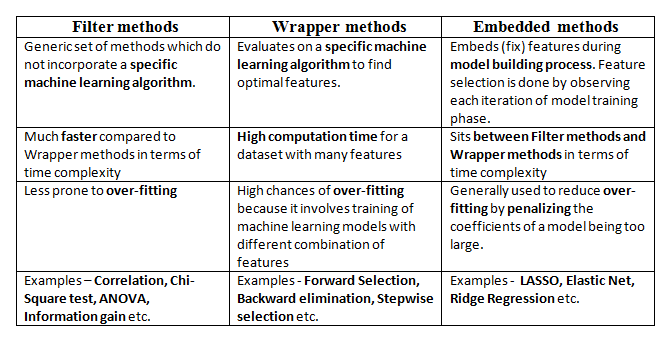
In this post, we will only discuss feature selection using Wrapper methods in Python.
Wrapper methods
In wrapper methods, the feature selection process is based on a specific machine learning algorithm that we are trying to fit on a given dataset.
It follows a greedy search approach by evaluating all the possible combinations of features against the evaluation criterion. The evaluation criterion is simply the performance measure which depends on the type of problem, for e.g. For regression evaluation criterion can be p-values, R-squared, Adjusted R-squared, similarly for classification the evaluation criterion can be accuracy, precision, recall, f1-score, etc. Finally, it selects the combination of features that gives the optimal results for the specified machine learning algorithm.

Most commonly used techniques under wrapper methods are:
Forward selection
Backward elimination
Bi-directional elimination(Stepwise Selection)
Too much theory so far. Now let us discuss wrapper methods with an example of the Boston house prices dataset available in sklearn. The dataset contains 506 observations of 14 different features. The dataset can be imported using the load_boston()function available in the sklearn.datasets module.
Python Code:
from sklearn.datasets import load_boston
import warnings
warnings.filterwarnings('ignore')
boston = load_boston()
print(boston.data.shape)         # for dataset dimension
print(boston.feature_names)      # for feature names
print(boston.target)             # for target variable
print(boston.DESCR)
Let’s convert this raw data into a data frame including target variable and actual data along with feature names.
import pandas as pd
bos = pd.DataFrame(boston.data, columns = boston.feature_names)
bos['Price'] = boston.target
X = bos.drop("Price", 1)       # feature matrix
y = bos['Price']               # target feature
bos.head()
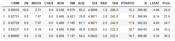
Here, the target variable is Price. We will be fitting a regression model to predict Price by selecting optimal features through wrapper methods.
1. Forward selection
In forward selection, we start with a null model and then start fitting the model with each individual feature one at a time and select the feature with the minimum p-value. Now fit a model with two features by trying combinations of the earlier selected feature with all other remaining features. Again select the feature with the minimum p-value. Now fit a model with three features by trying combinations of two previously selected features with other remaining features. Repeat this process until we have a set of selected features with a p-value of individual features less than the significance level.
In short, the steps for the forward selection technique are as follows :
Choose a significance level (e.g. SL = 0.05 with a 95% confidence).
Fit all possible simple regression models by considering one feature at a time. Total ’n’ models are possible. Select the feature with the lowest p-value.
Fit all possible models with one extra feature added to the previously selected feature(s).
Again, select the feature with a minimum p-value. if p_value < significance level then go to Step 3, otherwise terminate the process.
Now let us perform the same on Boston house price data.
def forward_selection(data, target, significance_level=0.05):
    initial_features = data.columns.tolist()
    best_features = []
    while (len(initial_features)>0):
        remaining_features = list(set(initial_features)-set(best_features))
        new_pval = pd.Series(index=remaining_features)
        for new_column in remaining_features:
            model = sm.OLS(target, sm.add_constant(data[best_features+[new_column]])).fit()
            new_pval[new_column] = model.pvalues[new_column]
        min_p_value = new_pval.min()
        if(min_p_value<significance_level):
            best_features.append(new_pval.idxmin())
        else:
            break
    return best_features
This above function accepts data, target variable, and significance level as arguments and returns the final list of significant features based on p-values through forward selection.
forward_selection(X,y)
#OUTPUT
['LSTAT',
'RM',
'PTRATIO',
'DIS',
'NOX',
'CHAS',
'B',
'ZN',
'CRIM',
'RAD',
'TAX']
Implementing Forward selection using built-in functions in Python:
mlxtend library contains built-in implementation for most of the wrapper methods based feature selection techniques. SequentialFeatureSelector() function comes with various combinations of feature selection techniques.
#importing the necessary libraries
from mlxtend.feature_selection import SequentialFeatureSelector as SFS
from sklearn.linear_model import LinearRegression
# Sequential Forward Selection(sfs)
sfs = SFS(LinearRegression(),
          k_features=11,
          forward=True,
          floating=False,
          scoring = 'r2',
          cv = 0)
SequentialFeatureSelector() function accepts the following major arguments :
LinearRegression() is an estimator for the entire process. Similarly, it can be any classification based algorithm.
k_features indicates the number of features to be selected. It can be any random value, but the optimal value can be found by analyzing and visualizing the scores for different numbers of features.
forward and floating arguments for different flavors of wrapper methods, here, forward = True and floating = False are for forward selection technique.
The scoring argument specifies the evaluation criterion to be used. For regression problems, there is only r2 score in default implementation. Similarly for classification, it can be accuracy, precision, recall, f1-score, etc.
cv argument is for k-fold cross-validation.
Now let’s fit the above-defined feature selector on the Boston house price dataset.
sfs.fit(X, y)
sfs.k_feature_names_     # to get the final set of features
#OUTPUT
('CRIM',
'ZN',
'CHAS',
'NOX',
'RM',
'DIS',
'RAD',
'TAX',
'PTRATIO',
'B',
'LSTAT')
2. Backward elimination
In backward elimination, we start with the full model (including all the independent variables) and then remove the insignificant feature with the highest p-value(> significance level). This process repeats again and again until we have the final set of significant features.
In short, the steps involved in backward elimination are as follows:
Choose a significance level (e.g. SL = 0.05 with a 95% confidence).
Fit a full model including all the features.
Consider the feature with the highest p-value. If the p-value > significance level then go to Step 4, otherwise terminate the process.
Remove the feature which is under consideration.
Fit a model without this feature. Repeat the entire process from Step 3.
Now let us perform the same on Boston house price data.
def backward_elimination(data, target,significance_level = 0.05):
    features = data.columns.tolist()
    while(len(features)>0):
        features_with_constant = sm.add_constant(data[features])
        p_values = sm.OLS(target, features_with_constant).fit().pvalues[1:]
        max_p_value = p_values.max()
        if(max_p_value >= significance_level):
            excluded_feature = p_values.idxmax()
            features.remove(excluded_feature)
        else:
            break
    return features
This above function returns the final list of significant features based on p-values through backward elimination.
# OUTPUT
['CRIM',
'ZN',
'CHAS',
'NOX',
'RM',
'DIS',
'RAD',
'TAX',
'PTRATIO',
'B',
'LSTAT']
Implementing Backward elimination using built-in functions in Python:
The same SequentialFeatureSelector()function can be used to perform backward elimination by disabling the forward argument.
#Sequential backward selection(sbs)
sbs = SFS(LinearRegression(),
         k_features=11,
         forward=False,
         floating=False,
         cv=0)
sbs.fit(X, y)
sbs.k_feature_names_
# OUTPUT
('CRIM',
'ZN',
'CHAS',
'NOX',
'RM',
'DIS',
'RAD',
'TAX',
'PTRATIO',
'B',
'LSTAT')
Additional Note
Here we are directly using the optimal value of k_features argument in both forward selection and backward elimination. In order to find out the optimal number of significant features, we can use the hit and trial method for different values of k_features and make the final decision by plotting it against the model performance.
sfs1 = SFS(LinearRegression(),
         k_features=(3,11),
         forward=True,
         floating=False,
         cv=0)
sfs1.fit(X, y)
The same visualization can be achieved through plot_sequential_feature_selection()function available in mlxtend.plotting module.
from mlxtend.plotting import plot_sequential_feature_selection as plot_sfs
import matplotlib.pyplot as plt
fig1 = plot_sfs(sfs1.get_metric_dict(), kind='std_dev')
plt.title('Sequential Forward Selection (w. StdErr)')
plt.grid()
plt.show()
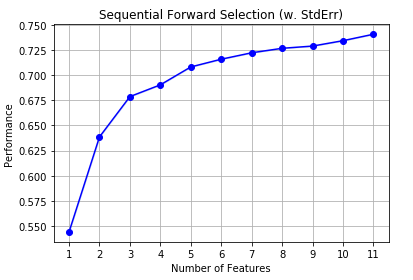
Here, on the y-axis, the performance label indicates the R-squared values for the different numbers of features.
3. Bi-directional elimination(Step-wise Selection)
It is similar to forward selection but the difference is while adding a new feature it also checks the significance of already added features and if it finds any of the already selected features insignificant then it simply removes that particular feature through backward elimination.
Hence, It is a combination of forward selection and backward elimination.
In short, the steps involved in bi-directional elimination are as follows:
Choose a significance level to enter and exit the model (e.g. SL_in = 0.05 and SL_out = 0.05 with 95% confidence).
Perform the next step of forward selection (newly added feature must have p-value < SL_in to enter).
Perform all steps of backward elimination (any previously added feature with p-value>SL_out is ready to exit the model).
Repeat steps 2 and 3 until we get a final optimal set of features.
Let us perform the same on Boston house price data.
def stepwise_selection(data, target,SL_in=0.05,SL_out = 0.05):
    initial_features = data.columns.tolist()
    best_features = []
    while (len(initial_features)>0):
        remaining_features = list(set(initial_features)-set(best_features))
        new_pval = pd.Series(index=remaining_features)
        for new_column in remaining_features:
            model = sm.OLS(target, sm.add_constant(data[best_features+[new_column]])).fit()
            new_pval[new_column] = model.pvalues[new_column]
        min_p_value = new_pval.min()
        if(min_p_value<SL_in):
            best_features.append(new_pval.idxmin())
            while(len(best_features)>0):
                best_features_with_constant = sm.add_constant(data[best_features])
                p_values = sm.OLS(target, best_features_with_constant).fit().pvalues[1:]
                max_p_value = p_values.max()
                if(max_p_value >= SL_out):
                    excluded_feature = p_values.idxmax()
                    best_features.remove(excluded_feature)
                else:
                    break
        else:
            break
    return best_features
This above function returns the final list of significant features based on p-values through bi-directional elimination.
stepwise_selection(X,y)
# OUTPUT
['LSTAT',
'RM',
'PTRATIO',
'DIS',
'NOX',
'CHAS',
'B',
'ZN',
'CRIM',
'RAD',
'TAX']
Implementing bi-directional elimination using built-in functions in Python:
The same SequentialFeatureSelector()function can be used to perform backward elimination by enabling forward and floating arguments.
# Sequential Forward Floating Selection(sffs)
sffs = SFS(LinearRegression(),
         k_features=(3,11),
         forward=True,
         floating=True,
         cv=0)
sffs.fit(X, y)
sffs.k_feature_names_
# OUTPUT
('CRIM',
'ZN',
'CHAS',
'NOX',
'RM',
'DIS',
'RAD',
'TAX',
'PTRATIO',
'B',
'LSTAT')
End Notes
In this article, we saw different kinds of Wrapper methods for feature selection with implementation using mlxtend library in Python.
A Data Science professional with 7.5 years of experience in data science, machine learning, and programming. Hands-on experience in different domains like data analytics, deep learning, big data, and natural language processing.


Dear Vikas, You may want to consider the images you use on Linkedin to make your point on models with or without feature engineering. the two I've recently seen depict female models and male data scientists, which is currently not considered particularly appropriate, and in fact sexist. If you want to reach customers of any kind, I suggest you reconsider the images. have a nice day
Can forward, backward, or stepwise selection be applied also with another regression than the linear one ? Like why not polyomial regression whereby the polynomial degree would be another hyperparameter ? Or why not even random forest ? Thank you.
Very good article, your job is very appreciated! One advice would be if you could add some references in the end, then the article would be a complete picture and even more useful. All the best!