Bellman Optimality Equation in Reinforcement Learning
Introduction
In this article, first, we will discuss some of the basic terminologies of Reinforcement Learning, then we will further understand the crux behind the most commonly used equations in Reinforcement Learning, and then we will dive deep into understanding the Bellman Optimality Equation.
The aim of this article is to give an intuition about Reinforcement Learning as well as what the Bellman Optimality Equation is and how it is used in solving Reinforcement Learning problems. This article does not contain complex mathematical explanations for the equations. So don’t worry.
This article was published as a part of the Data Science Blogathon.
Table of contents
What is Reinforcement Learning?
Reinforcement Learning (RL)in Dynamic Programming is a paradigm in machine learning that encompasses the concept of agents interacting with environments to learn optimal actions through trial and error. Analogous to a child learning to walk or ride a bicycle, RL entails navigating a dynamic environment with partial supervision, akin to a child’s experience of receiving occasional guidance but largely learning through self-correction.
In RL, agents operate within environments, transitioning between states and taking actions to maximize cumulative rewards. The process unfolds over an infinite horizon, where each action influences subsequent states, creating a successor state based on the chosen action. To guide decision-making, agents employ policies dictating action selection strategies.
Policy iteration is a fundamental technique in RL, involving the iterative refinement of policies to converge on optimal solutions. This process entails evaluating policies through backup diagrams, recursively assessing state-action values to inform policy updates. Dynamic programming, a key approach in reinforcement learning, aids in policy evaluation and improvement, enabling agents to make informed decisions based on learned value functions.
Markov process underpins RL frameworks, characterized by state transitions governed by probabilities, facilitating decision-making in uncertain environments. Dynamic programming techniques are often employed to solve Markov decision processes efficiently, enabling agents to make optimal decisions even in complex environments.
Optimal actions are sought through iterative policy refinement, where agents strive to maximize cumulative rewards over time. Neural networks play a crucial role in RL, enabling agents to approximate value functions or policies, enhancing decision-making capabilities.
At its core, RL embodies a recursive relationship between actions, states, and rewards, where agents iteratively learn from experience to optimize decision-making processes. By navigating environments and adapting to feedback, RL agents emulate the trial-and-error learning observed in natural systems, fostering autonomous and adaptive behavior.
Agent
The agent in RL is an entity that tries to learn the best way to perform a specific task. In our example, the child is the agent who learns to ride a bicycle.
Action
The action in RL is what the agent does at each time step. In the example of a child learning to walk, the action would be “walking”.
State
The state in RL describes the current situation of the agent. After doing performing an action, the agent can move to different states. In the example of a child learning to walk, the child can take the action of taking a step and move to the next state (position).
Rewards
The rewards in RL is nothing but a kind of feedback that is given to the agent based on the action of the agent. If the action of the agent is good and can lead to winning or a positive side then a positive reward is given and vice versa. This is the same as if after successfully riding a bicycle for more amount of time, keeping balance the elder ones of child applauds him/her indicating the positive feedback.
Environment
The environment in RL refers to the outside world of an agent or physical world in which the agent operates.
Reinforcement learning (RL) is an area of machine learning concerned with how intelligent agents ought to take actions in an environment in order to maximize the notion of cumulative reward. Reinforcement learning is one of three basic machine learning paradigms, alongside supervised learning and unsupervised learning.
Now, the above definition taken from Wikipedia should make sense to some extent. Let us now understand the most common equations used in RL.
In RL, the agent selects an action from a given state, which results in transitioning to a new state, and the agent receives rewards based on the chosen action. This process happens sequentially which creates a trajectory that represents the chain/sequence of states, actions, and rewards. The goal of an RL agent is to maximize the total amount of rewards or cumulative rewards that are received by taking actions in given states.
For easy understanding of Dynamic Programming equations, we will define some notations. We denote a set of states as S, a set of actions as A, and a set of rewards as R. At each time step t = 0, 1, 2, …, some representation of the environment’s state St ∈ S is received by the agent. According to this state, the agent selects an action At ∈ A which gives us the state-action pair (St, At). In the next time step t+1, the transition of the environment happens and the new state St+1 ∈ S is achieved. At this time step t+1, a reward Rt+1 ∈ R is received by the agent for the action At taken from state St.
As we mentioned above that the goal of the agent is to maximize the cumulative rewards, we need to represent this cumulative reward in a formal way to use it in the calculations. We can call it as Expected Return and can be represented as,
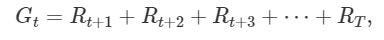
Expected Return for Episodic Tasks (Source)
The above Dynamic Programming equation works for episodic tasks. For continuing tasks, we need to update this equation as we don’t have a limit of time step T in continuing tasks. Discount factor γ is introduced here which forces the agent to focus on immediate rewards instead of future rewards. The value of γ remains between 0 and 1.
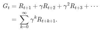
Expected Return for Continuing Tasks (Source)
Policies
Policy in RL decides which action will the agent take in the current state. In other words, It tells the probability that an agent will select a specific action from a specific state.
Policies tell how probable it is for an agent to select any action from a given state.
Defining technically,
Policy is a function that maps a given state to probabilities of selecting each possible action from the given state.
If at time t, an agent follows policy π, then π(a|s) becomes the probability that the action at time step t is At=a if the state at time step t is St=s. The meaning of this is, the probability that an agent will take an action a in state s is π(a|s) at time t with policy π.
Value Functions
The value of Dynamic functions are nothing but a simple measure of how good it is for an agent to be in a given state, or how good it is for the agent to perform a given action in a given state.
There are two kinds of value functions which are described below:
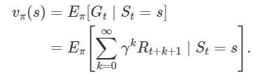
State Value Function (Source)
The state-value function for policy π denoted as vπ determines the goodness of any given state for an agent who is following policy π. This function gives us the value which is the expected return starting from state s at time step t and following policy π afterward.
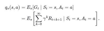
Action Value Function (Source)
The action-value function mentioned above determines the goodness of the action taken by the agent from a given state for policy π. This function gives the value which is the expected return starting from state s at time step t, with action a, and following policy π afterward. The output of this function is also called as Q-value where q stands for Quality. Note that in the state-value function, we did not consider the action taken by the agent.
Now that we have defined the basic equations for solving an RL problem, our focus now should be to find an optimal solution (optimal policy in the case of RL). Therefore let us go through the optimality domain of RL and along the way, we will encounter the Bellman Optimality Equation also.
The policy π can be considered better than or same as the policy π′ if the expected return of policy π is greater than or equal to the expected return of policy π′ for all states. Such policy π is called Optimal Policy.
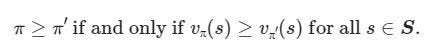
Optimal Policy (Source)
The optimal policy should have an associated optimal state-value function or action-value function.
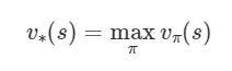
Optimal State-Value Function (Source)
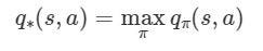
Optimal Action-Value Function (Source)
The optimal state-value function v∗ yields the largest expected return feasible for each of the state s with any policy π. And the optimal action-value function q∗ yields the largest expected return feasible for each state-action pair (s, a) with any policy π.
Bellman Optimality Equation
The optimal action-value function q∗ satisfies the below-given equation. This is a fundamental property of the optimal action-value function.
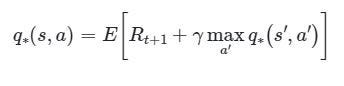
Bellman Optimality Equation (Source)
This equation is called Bellman Optimality Equation. Now, what this equation has to do with optimality in RL? The answer is in the next paragraph.
This equation tells that, at time t, for any state-action pair (s, a), the expected return from starting state s, taking action a, and with the optimal policy afterward will be equal to the expected reward Rt+1 we can get by selecting action a in state s, in addition with the maximum of “expected discounted return” that is achievable of any (s′, a′) where (s′, a′) is a potential next state-action pair.
Considering the agent following an optimal policy, the latter state s′ will be the state from we can take the best possible next action a′ at time t+1. This seems somewhat difficult to understand.
The essence is that this equation can be used to find optimal q∗ in order to find optimal policy π and thus a reinforcement learning algorithm can find the action a that maximizes q∗(s, a). That is why this equation has its importance.
The Optimal Value Function is recursively related to the Bellman Optimality Equation.
The above property can be observed in the equation as we find q∗(s′, a′) which denotes the expected return after choosing an action a in state s which is then maximized to gain the optimal Q-value.
Q-value Updation
During the training of an RL agent in order to determine the optimal policy, we need to update the Q-value (Output of the Action-Value Function) iteratively.
The Q-learning algorithm (which is nothing but a technique to solve the optimal policy problem) iteratively updates the Q-values for each state-action pair using the Bellman Optimality Equation until the Q-function (Action-Value function) converges to the optimal Q-function, q∗. This process is called Value-Iteration.
To make the Q-value eventually converge to an optimal Q-value q∗, what we have to do is —for the given state-action pair, we have to make the Q-value as near as we can to the right-hand side of the Bellman Optimality Equation. For this, the loss between the Q-value and the optimal Q-value for the given state-action pair will be compared iteratively, and then each time we encounter the same state-action pair, we will update the Q-value, again and again, to reduce the loss. The loss can be given as q∗(s, a)-q(s, a).
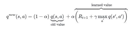
Q-Value Updation (Source)
We can not overwrite the newly computed Q-value with the older value. Instead, we use a parameter called learning rate denoted by α, to determine how much information of the previously computed Q-value for the given state-action pair we retain over the newly computed Q-value calculated for the same state-action pair at a later time step. The higher the learning rate, the more quickly the agent will adopt the newly computed Q-value. Therefore we need to take care of the trade-off between new and old Q-value using the appropriate learning rate.
After coming this far, you should have got an idea of why and how the Bellman Optimality Equation is used in RL and you should have reinforced your learning on Reinforcement Learning. Thank you for reading this article.
Conclusion
In the realm of reinforcement learning, understanding the Bellman Optimality Equation is paramount. It delineates the optimal value function, guiding agents towards decision-making that maximizes cumulative rewards. Through Q-learning and iterative updates, agents converge to the optimal policy, unraveling the intricate dynamics of decision-making in complex environments. As the quest for optimal solutions persists, the Bellman Optimality Equation stands as a beacon, illuminating the path towards intelligent agent-based systems, where actions are orchestrated to navigate the nuances of uncertainty and complexity inherent in real-world scenarios.
References:
[1] NPTEL Course on RL [2] RL Course by David Silver [3] DeepLizard RLFrequently Asked Questions
A. An optimal policy has the property that no matter where the initial decision is the remaining decisions constitute an optimal policy. Bellman 1957, Chappe. I.
A. Bellman equations : |St= = E [T + G+ |T +1 |T = – s]= E[Rt+1 + V (ST + +1|T +1] |T=s]
A. The principle of Bellman is the primary principle of determining optimal solutions. DP computes an optimal solution for the decision variables.
A. Bellman’s equation explains that value of a state equals the expectation immediately of reward plus a discount value for the next. The underlying code is used in value iterative and other dynamic programmers that solve MDP problems. July 8, 2020


Hututu land hututu by vinay distic JD ho DL to do to to do XL XL Clapp Flatt faizi calculation history happy that hai