Introduction
Reinforcement learning (RL) is an area of machine learning concerned with how intelligent agents ought to take actions in an environment in order to maximize the notion of cumulative reward. (Wiki)
Everyone heard when DeepMind announced its milestone project AlphaGo –
AlphaGo is the first computer program to defeat a professional human Go player, the first to defeat a Go world champion, and is arguably the strongest Go player in history.
This alone says a lot about how powerful the program itself is but how did they achieve it? They did it through novel approaches in Reinforcement learning!
And it’s not just fixated on games, the applications range from –
- Self-driving cars
- industry automation
- trading and finance
- NLP (Natural Language Processing)
- Healthcare
- News Recommendation
- Real-time bidding (Marketing and Advertising)
- Robotics
This article was published as a part of the Data Science Blogathon
Table of contents
- What is Reinforcement Lerning?
- Fundamentals of Reinforcement Learning
- Rough Idea to relate Reinforcement Learning problems
- OpenAI Gym for Training Reinforcement Learning Agents
- Cartpole-Balancing using Random Agent
- Popular Algorithms in Reinforcement Learning
- Start coding our DQN algorithm
- Reinforcement Learning Libraries in Python
- Challenges in Reinforcement Learning
- Frequently Asked Questions?
What is Reinforcement Lerning?
Reinforcement Learning is a subset of machine learning focused on self-training agents through reward and punishment mechanisms. Agents aim to maximize rewards and minimize punishment by selecting optimal actions based on observations within a given context. This approach reinforces positive behaviors and discourages negative ones. Agents perceive and interpret their environment, taking actions and interacting with it accordingly. By iteratively learning from these interactions, reinforcement learning enables agents to make informed decisions and navigate complex scenarios autonomously, making it a powerful paradigm in artificial intelligence.
Fundamentals of Reinforcement Learning
Let’s dig into the fundamentals of RL and review them step by step.
Key elements fundamental to RL
There are basically 4 elements – Agent, Environment, State-Action, Reward
Agent
An agent is a program that learns to make decisions. We can say that an agent is a learner in the RL setting. For instance, a badminton player can be considered an agent since the player learns to make the finest shots with timing to win the game. Similarly, a player in FPS games is an agent as he takes the best actions to improve his score on the leaderboard.
Environment
The playground of the agent is called the environment. The agent takes all the actions in the environment and is bound to be in it.
For instance, we discussed badminton players, here the court is the environment in which the player moves and takes appropriate shots. Same in the case of the FPS game, we have a map with all the essentials (guns, other players, ground, buildings) which is our environment to act for an agent.
State – Action
A state is a moment or instance in the environment at any point. Let’s understand it with the help of chess. There are 64 places with 2 sides and different pieces to move. Now this chessboard will be our environment and player, our agent. At some point after the start of the game, pieces will occupy different places in the board, and with every move, the board will differ from its previous situation. This instance of the board is called a state(denoted by s). Any move will change the state to a different one and the act of moving pieces is called action (denoted by a).
Reward
We have seen how taking actions change the state of the environment. For each action ‘a’ the agent takes, it receives a reward (feedback). The reward is simply a numerical value assigned which could be negative or positive with different magnitude.
Let’s take badminton example if the agent takes the shot which results in a positive score we can assign a reward as +10. But if it gets the shuttle inside his court then it will get a negative reward -10. We can further break rewards by giving small positive rewards(+2) for increasing the chances of a positive score and vice versa.
Rough Idea to relate Reinforcement Learning problems
Before we move on to the Math essentials, I’d like to give a bird-eye view of the reinforcement learning problem. Let’s take the analogy of training a pet to do few tricks. For every successful completion of the trick, we give our pet a treat. If the pet fails to do the same trick we don’t give him a treat. So, our pet will figure out what action caused it to receive a cookie and repeat that action. Thus, our pet will understand that completing a trick caused it to receive a treat and will attempt to repeat doing the tricks. Thus, in this way, our pet will learn a trick successfully while aiming to maximize the treats it can receive.
Here the pet was Agent, groundfloor our environment which includes our pet. Treats given were rewards and every action pet took landed him in a different state than the previous.
Markov Decision Process (MDP)
The Markov Decision Process (MDP) provides a mathematical framework for solving RL problems. Almost all RL problems can be modeled as an MDP. MDPs are widely used for solving various optimization problems. But to understand what MDP is, we’d have to understand Markov property and Markov Chain.
The Markov property and Markov chain
Markov Property is simply put – says that future states will not depend on the past and will solely depend on the present state. The sequence of these states (obey Markov property) is called Markov Chain.
Change from one state to another is called transition and the probability of it is transition probability. In simpler words, it means in every state we can have different choices(actions) to choose from. Each choice(action) will result in a different state and the probability of reaching the next state(s’) will be stored in our sequence.
Now, if we add rewards in Markov Chains we get a sequence with the state, transition probability, and rewards (The Markov Reward Process). If we further extend this to include actions it will become The Markov Decision Process. So, MDP is just a sequence of . We will learn more concepts on the go as we move further.
OpenAI Gym for Training Reinforcement Learning Agents
OpenAI is an AI research and deployment company whose goal is to ensure that artificial general intelligence benefits all of humanity. OpenAI provides a toolkit for training RL agents called Gym.
As we have learned that, to create an RL model we need to create an environment first. The gym comes into play here and helps us to create abstract environments to train our agents on it.
- Installing Gym
- Overview of Gym
- Creating an episode in the Gym environment
- Cart-Pole balancing with a random agent
Installing Gym
Its installation is simple using Pip. Though the latest version of Gym was just updated a few days ago after years, we can still use the 0.17 version.pip install gym
You can also clone it from the repository.git clone https://github.com/openai/gym
cd gym
pip install -e .
Creating our first environment using Gym
We will use pre-built (in Gym) examples. One can get explore all the agents from OpenAI gym documentation. Let’s start with Mountain Car.
First, we import Gymimport gym
To create an environment we use the ‘make’ function which required one parameter ID (pre-built ones can be found in the documentation)env = gym.make(‘CartPole-v0’)
To can see how our environment actually looks like using render function.env.render()
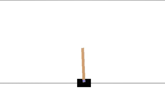
The goal here is to balance the pole as long as possible by moving the cart left or right.
To close rendered environment, simply useenv.close()
Cartpole-Balancing using Random Agent
import gym
env = gym.make('CartPole-v0')
env.reset()
for _ in range(1000):
     env.render()
     env.step(env.action_space.sample()) # take a random action env.close()
We created an environment, the first thing we do is to reset our environment to its default values. Then we ran it for 1000 timesteps by taking random actions. The ‘step’ function is basically transitioning our current state to the next state by taking the action our agent gives (in this case it was random).
Before moving deeper, let’s understand what are spaces!
Observations
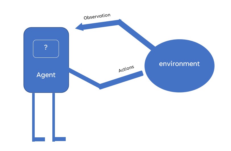
If we want to do better than just taking random actions, we’d have to understand what our actions are doing to the environment.
The environment’s step function returns what we need in the form of 4 values :
- observation (object): an environment-specific object representing the observation of our environment. For example, state of the board in a chess game, pixels as data from cameras or joints torque in robotic arms.
- reward (float): the amount of reward achieved by each action taken. It varies from env to env but the end goal is always to maximize our total reward.
- done (boolean): if it’s time to reset our environment again. Most of the tasks are divided into a defined episode (completion) and if done is true it means the env has completed the episode. For example, a player wins in chess or we lose all lives in the Mario game.
- info (dict): It is simply diagnostic information that is useful for debugging. The agent does not use this for learning, although it can be used for other purposes. If we want to extract some info from each timestep or episode it can be done through this.
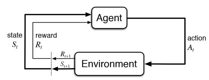
This is an implementation of the classic “agent-environment loop”. With each timestep, the agent chooses an action, and the environment returns an observation and a reward with info(not used for training).
The whole process starts by calling the reset() function, which returns an initial observation.
import gym

env = gym.make('CartPole-v0')

for i_episode in range(20):
    observation = env.reset()

    for t in range(100):
        env.render()  # Renders our cartpole environment
        print(observation)

        action = env.action_space.sample()  # Takes random action from action space
        observation, reward, done, info = env.step(action)

        if done:
            # Prints number of timesteps it took to finish the episode
            print("Episode finished after {} timesteps".format(t+1))
            break

env.close()
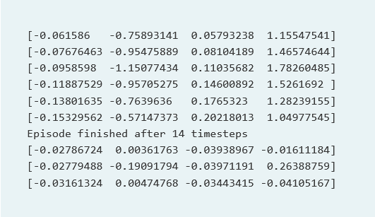
Now, what we see here is observation at each timestep, in Cartpole env observation is a list of 4 continuous values. While our actions are just 0 or 1. To check what is observation space we can simply call this function –
import gym

print(env.action_space) #type and size of action space #> Discrete(2)print(env.observation_space) #type and size of observation space #> Box(4,)
Discrete and box are the most common type of spaces in Gym env. Discrete as the name suggests has defined values while box consists of continuous values. Action values are as follows –
| Value | Action |
| 0 | Push cart towards the left |
| 1 | Push cart towards the right |
Meanwhile, the observation space is a Box(4,) with 4 continuous values denoting –
| 0.02002610 | -0.0227738 | 0.01257453 | 0.04411007 |
| Position of Cart | Velocity of Cart | Angle of Pole | The velocity of Pole at the tip |
Gym environments are not just restricted to text or cart poles, its wide range is as follows –
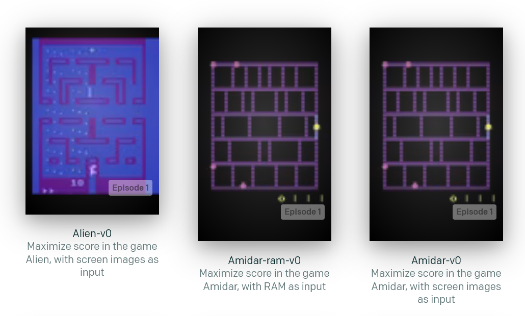
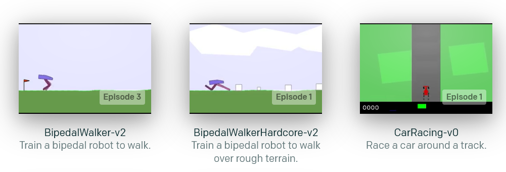
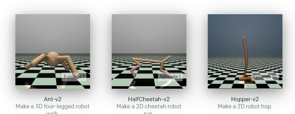
And many more… We can also create our own custom environment in the gym suiting to our needs.
Popular Algorithms in Reinforcement Learning
In this section, I will cover popular algorithms commonly used in Reinforcement Learning. Right after some basic concepts, it will be followed with implementation in python.
Deep Q Network
The objective of reinforcement learning is to find the optimal policy, that is, the policy that gives us the maximum return (the sum of total rewards of the episode). To compute policy we need to first compute the Q function. Once we have the Q function, then we can create a policy that selects the best action based on the maximum Q value. For instance, let’s assume we have two states A and B, we are in state A which has 4 choices, and corresponding to each choice(action) we have a Q value. In order to maximize returns, we follow the policy that has argmax (Q) for that state.
| State | Action | Value |
| A | left | 25 |
| A | Right | 35 |
| A | up | 12 |
| A | down | 6 |
We are using a neural network to approximate the Q value hence that network is called the Q network, and if we use a deep neural network to approximate the Q value, then it is called a deep Q network or (DQN).
Basic elements we need for understanding DQN is –
- Replay Buffer
- Loss Function
- Target Network
Replay Buffer
We know that the agent makes a transition from a state s to the next state 𝑠′ by performing some action a, and then receives a reward r. We can save this transition information in a buffer called a replay buffer or experience replay. Later we sample random batches from buffer to train our agent.
Loss Function
We learned that in DQN, our goal is to predict the Q value, which is just a continuous value. Thus, in DQN we basically perform a regression task. We generally use the mean squared error (MSE) as the loss function for the regression task. We can also use different functions to compute the error.
Target Network
There is one issue with our loss function, we need a target value to compute the losses but when the target is in motion we can no longer get stable values of y_i to compute loss, so here we use the concept of soft update. We create another network that updates slowly as compared to our original network and computes losses since now we have frozen values of y_i. It will be better understood with the code below.
Start coding our DQN algorithm
import random
import gym
import numpy as np
from collections import deque
from tensorflow.keras.models import Sequential
from tensorflow.keras.layers import Flatten, Conv2D, MaxPooling2D , Dense, Activation
from tensorflow.keras.optimizers import Adam
Setting up the environment, it is advisable to check the game once to get a better idea of the working
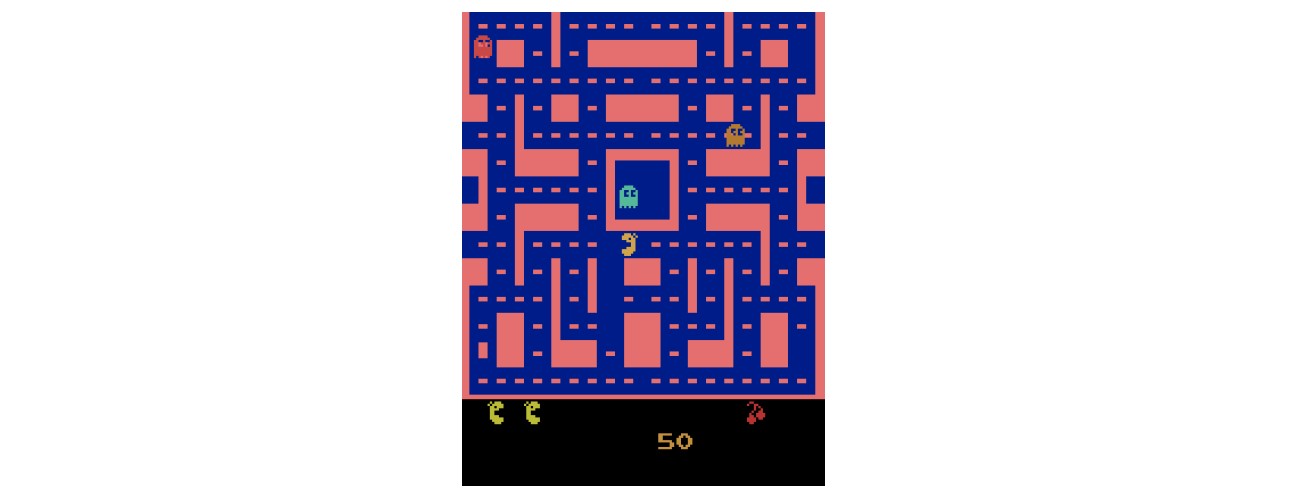
env = gym.make("MsPacman-v0")

state_size = (88, 80, 1) #defining state size as image input pixels

action_size = env.action_space.n     #number of actions to be taken
Pre-processing to feed image in our CNN
color = np.array([210, 164, 74]).mean()
def preprocess_state(state): #creating a function to pre-process raw image from game

     #cropping the image and resizing it
     image = state[1:176:2, ::2]

     #converting the image to greyscale
     image = image.mean(axis=2)

     #improving contrast
     image[image==color] = 0

     #normalize
     image = (image - 128) / 128 - 1

     #reshape and returning the image in format of state space
     image = np.expand_dims(image.reshape(88, 80, 1), axis=0)

     return image
We need to pre-process the raw image from the game, like removing color, cropping to the desired area, resizing it to state space as we defined previously.
Building DQN class
cclass DQN:
    def __init__(self, state_size, action_size):

        #defining state size
        self.state_size = state_size

        #number of actions
        self.action_size = action_size

        #Maximum size of replay buffer for our agent
        self.replay_buffer = deque(maxlen=5000)
        #gamma is our discount factor
        self.gamma = 0.9
        #epsilon of 0.8 denotes we get 20% random decision
        self.epsilon = 0.8

        #define the update rate at which we update the target network
        self.update_rate = 1000
        #building our main Neural Network
        self.main_network = self.build_network()
        #building our target network (same as our main network)
        self.target_network = self.build_network()
        #copying weights to target network
        self.target_network.set_weights(self.main_network.get_weights())
    def build_network(self):
        #creating a neural net
        model = Sequential()
        model.add(Conv2D(32, (8, 8), strides=4, padding='same', input_shape=self.state_size))
        model.add(Activation('relu'))

        #adding hidden layer 1
        model.add(Conv2D(64, (4, 4), strides=2, padding='same'))
        model.add(Activation('relu'))

        #adding hidden layer 2
        model.add(Conv2D(64, (3, 3), strides=1, padding='same'))
        model.add(Activation('relu'))
        model.add(Flatten())

        #feeding flattened map into our fully connected layer
        model.add(Dense(512, activation='relu'))
        model.add(Dense(self.action_size, activation='linear'))

        #compiling model using MSE loss with adam optimizer
        model.compile(loss='mse', optimizer=Adam())
        return model
    #we sample random batches of data, to store whole transition in buffer
    def  store_transistion( self, state, action, reward, next_state, done ):
        self.replay_buffer.append(( state, action, reward, next_state, done))
    # defining epsilon greedy function so our agent can tackle exploration vs exploitation issue
    def epsilon_greedy(self, state):
        #whenever a random value < epsilon we take random action
        if random.uniform(0,1) < self.epsilon:
            return np.random.randint(self.action_size)

        #then we calculate the Q value
        Q_values = self.main_network.predict(state)

        return np.argmax(Q_values[0])
    #this is our main training function
    def train(self, batch_size):
        #we sample a random batch from our replay buffer to train the agent on past actions
        minibatch = random.sample(self.replay_buffer, batch_size)

        #compute Q value using target network
        for state, action, reward, next_state, done in minibatch:

        #we calculate total expected rewards from this policy if episode is not terminated
            if not done:
                target_Q = (reward + self.gamma * np.amax(self.target_network.predict(next_state)))
            else:
                target_Q = reward
        #we compute the values from our main network and store it in Q_value
            Q_values = self.main_network.predict(state)

        #update the target Q value for losses
            Q_values[0][action] = target_Q

        #training main network
            self.main_network.fit(state, Q_values, epochs=1, verbose=0)

    #update the target network weights by copying from the main network
    def update_target_network(self):
        self.target_network.set_weights(self.main_network.get_weights()
Now we train our network after defining the values of hyper-paramsnum
num_episodes = 500              #number of episodes to train agent on
num_timesteps = 20000           #number of timesteps to be taken in each episode (until done)
batch_size = 8                  #taking batch size as 8
num_screens = 4                 #number of past game screens we want to use
dqn = DQN(state_size, action_size)    #initiating the DQN class
done = False                    #setting done to false (start of episode)
time_step = 0                   #begining of timestep
for i in range(num_episodes):
    #reset total returns to 0 before starting each episode
    Return = 0
    #preprocess the raw image from game
    state = preprocess_state(env.reset())

    for t in range(num_timesteps):
        env.render()               #render the env
        time_step += 1             #increase timestep with each loop

        #updating target network
        if time_step % dqn.update_rate == 0:
            dqn.update_target_network()

        #selection of action based on epsilon-greedy strategy
        action = dqn.epsilon_greedy(state)

        #saving the output of env after taking 'action'
        next_state, reward, done, _ = env.step(action)

        #Pre-process next state
        next_state = preprocess_state(next_state)
        #storing transition to be used later via replay buffer
        dqn.store_transistion(state, action, reward, next_state, done)
        #updating current state to next state
        state = next_state

        #calculating total reward
        Return += reward

        if done:
            print('Episode: ',i, ',' 'Return', Return) #if episode is completed terminate the loop
            break

        #we train if the data in replay buffer is greater than batch_size
        #for first 1-batch_size we take random actions
        if len(dqn.replay_buffer) > batch_size:
            dqn.train(batch_size)
Results – Agent learned to play the game successfully.
DDPG (Deep Deterministic Policy Gradient)
DQN works only for discrete action space but it’s not always the case that we need discrete values. What if we want continuous action output? to overcome this situation, we start with DDPG (Timothy P. Lillicrap 2015) to deal with when both state and action space is continuous. The idea of replay buffer, target functions, loss functions will be taken from DQN but with novel techniques which I will explain in this section.
Now let’s make an environment where we have a budget which we want to spend it on Facebook and Instagram advertisement. Our goal is to maximize the sales from these spends. So, all we need to create the basic environment in python is –
class AdSpendEnv(gym.Env):
def __init__(self, budget, seed=None):
self.budget = budget
self.observation_space = spaces.Box(low=0, high=budget, shape=(1,), dtype=np.float32)
self.action_space = spaces.Box(low=0, high=budget, shape=(1,), dtype=np.float32)
self.seed(seed)
def seed(self, seed=None):
self.np_random, seed = seeding.np_random(seed)
return [seed]
def step(self, action):
# Placeholder implementation; replace with your logic
new_state = np.array([0.0]) # Placeholder
reward = 0 # Placeholder
done = False # Placeholder
info = {} # Placeholder
return new_state, reward, done, info
def reset(self):
# Placeholder implementation; replace with your logic
initial_spends = np.zeros(1) # Placeholder
self.budget = budget # Placeholder
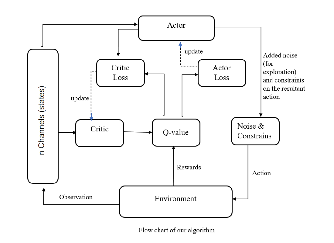
return initial_spendsNow, we move on to the core Actor-critic method. The original paper explains this concept quite well, but here is a rough idea. The actor takes a decision based on a policy, critic evaluates state-action pair, and gives it a Q value which is assigned to each pair. If the state-action pair is good enough according to critics, it will have a higher Q value (more preferable) and vice versa.
Critic Network
#creating class for critic network
class CriticNetwork(nn.Module):
    def __init__(self, beta):
        super(CriticNetwork, self).__init__()

        #fb, insta as state of 2 dim
        self.input_dims = 2

        #hidden layers with 256 N
        self.fc1_dims = 256

        #hidden layers with 256 N
        self.fc2_dims = 256

        #fb, insta spends as 2 actions to be taken
        self.n_actions = 2

        # state +  action as fully connected layer
        self.fc1 = nn.Linear( 2 + 2, self.fc1_dims )

        #adding hidden layers
        self.fc2 = nn.Linear(self.fc1_dims, self.fc2_dims)

        #final Q value from network
        self.q1 = nn.Linear(self.fc2_dims, 1)

        #using adam optimizer with beta as learning rate
        self.optimizer = optim.Adam(self.parameters(), lr=beta)

        #device available to train on CPU/GPU
        self.device = T.device('cuda' if T.cuda.is_available() else 'cpu')

        #assigning device
        self.to(self.device)
    #Creating Critic Network with state and action as input
    def CriticNetwork(self, state, action):

        #concatinating state and action before feeding to Neural Net
        q1_action_value = self.fc1(T.cat([state, action], dim=1 ))
        q1_action_value = F.relu(q1_action_value)

        #adding hidden layer
        q1_action_value = self.fc2(q1_action_value)
        q1_action_value = F.relu(q1_action_value)

        #getting final Q value
        q1 = self.q1(q1_action_value)
        return q1
Now we move to actor-network, we created a similar network but here are some key points which you must remember while making the actor.
- Weight initialization is not necessary but generally, if we provide initialization it tends to learn faster.
- Choosing an optimizer is very very important and results can vary from the optimizer to optimizer.
- Now, how to choose the last activation function solely depends on what kind of action-space, you are using, for example, if it is small and all values are like [-1,-2,-3] to [1,2,3] you can go ahead and tanh (squashing) function, but if you have [-2,-40,-230] to [2,60,560] you might want to change the activation function or create a wrapper.
Actor-Network
class ActorNetwork(nn.Module):

    #creating actor Network
    def __init__(self, alpha):
        super(ActorNetwork, self).__init__()

        #fb and insta as 2 input state dim
        self.input_dims = 2

        #first hidden layer dimension
        self.fc1_dims = fc1_dims

        #second fully connected layer dimension
        self.fc2_dims = fc2_dims

        #total number of actions
        self.n_actions = 2

        #connecting fully connected layers
        self.fc1 = nn.Linear(self.input_dims, self.fc1_dims)
        self.fc2 = nn.Linear(self.fc1_dims, self.fc2_dims)

        #final output as number of action values we need (2)
        self.mu = nn.Linear(self.fc2_dims, self.n_actions)

        #using adam as optimizer
        self.optimizer = optim.Adam(self.parameters(), lr=alpha)

        #setting up device (CPU or GPU) to be used for computation
        self.device = T.device('cuda' if  T.cuda.is_available() else  "cpu")
        self.to(self.device) #connecting the device
    def forward(self, state):

        #taking state as input to our fully connected layer
        prob = self.fc1(state)

        #adding activation layer
        prob = F.relu(prob)

        #adding second layer
        prob = self.fc2(prob)
        prob = F.relu(prob)

        #fixing each output between 0 and 1
        mu = T.sigmoid(self.mu(prob))

        return mu
Note: We used 2 hidden layers since our action space was small and our environment was not very complex. Authors of DDPG used 400 and 300 neurons for 2 hidden layers but we can increase at the cost of computation power.
Just like gym env, agent has some conditions too. We initialized our target networks with same weights as our original (A-C) networks. Since we are chasing a moving target, target networks create stability and helps original networks to train.
We initialize all the basic requirements, as you might have noticed we have a loss function parameter too. We can use different loss functions and choose whichever works best (can be L1 smooth loss), paper used mse loss, so we will go ahead and use it as default.
Here we include the ‘choose action’ function, you can create an evaluation function as well to cross-check values that outputs action space without noise.
‘Update parameter’ function, now this is where we do soft (target networks) and hard updates (original networks, complete copy). Here it takes only one parameter Tau, this is similar to how we think of learning rate.
It is used to soft update our target networks and in the paper, they found the best tau to be 0.001 and it usually is the best across different papers.
class Agent(object):

     #binding everything we did till now
        def __init__( self, alpha , beta, input_dims= 2, tau, env, gamma=0.99, n_actions=2,
                        max_size=1000000,  batch_size=64):

        #fixing discount rate gamma
        self.gamma = gamma

        #for soft updating target network, fix tau
        self.tau = tau

        #Replay buffer with max number of transitions to store
        self.memory = ReplayBuffer(max_size)

        #batch size to take from replay buffer
        self.batch_size = batch_size

        #creating actor network using learning rate alpha
        self.actor = ActorNetwork(alpha)

        #creating target network with same learning rate
        self.target_actor = ActorNetwork(alpha)

        #creating critic network with beta as learning rate
        self.target_critic = CriticNetwork(beta)

        #adjusting scale as std for adding noise
        self.scale = 1.0
        self.noise = np.random.normal(scale=self.scale,size=(n_actions))

        #hard updating target network weights to be same
        self.update_network_parameters(tau=1)

    #this function helps to retrieve actions by adding noise to output network
    def choose_action(self, observation):

        self.actor.eval() #get actor in eval mode

        #convert observation state to tensor for calcualtion
        observation = T.tensor(observation, dtype=T.float).to(self.actor.device)

        #get the output from actor network
        mu = self.actor.forward(observation).to(self.actor.device)

        #add noise to our output from actor network
        mu_prime = mu + T.tensor(self.noise(),dtype=T.float).to(self.actor.device)

        #set back to training mode
        self.actor.train()

        #get the final results as array
        return mu_prime.cpu().detach().numpy()

    #training our actor and critic network from memory (Replay buffer)
    def learn(self):

        #if batch size is not filled then do not train
        if self.memory.mem_cntr < self.batch_size:
            return

        #otherwise take a batch from replay buffer
        state, action, reward, new_state, done= self.memory.sample_buffer(self.batch_size)

        #convert all values to tensors

        reward = T.tensor(reward, dtype=T.float).to(self.critic.device)
        done = T.tensor(done).to(self.critic.device)
        new_state = T.tensor(new_state, dtype=T.float).to(self.critic.device)
        action = T.tensor(action, dtype=T.float).to(self.critic.device)
        state = T.tensor(state, dtype=T.float).to(self.critic.device)

        #set netowrks to eval mode
        self.target_actor.eval()
        self.target_critic.eval()
        self.critic.eval()

        #fetch the output from the target network
        target_actions = self.target_actor.forward(new_state)

        #get the critic value from both networks
        critic_value_ = self.target_critic.forward(new_state, target_actions)
        critic_value = self.critic.forward(state, action)

        #now we will calculate total expected reward from this policy
        target = []
        for j in range(self.batch_size):
            target.append(reward[j] + self.gamma*critic_value_[j]*done[j])

        #convert it to tensor on respective device(cpu or gpu)
        target = T.tensor(target).to(self.critic.device)
        target = target.view(self.batch_size, 1)

        #to train critic value set it to train mode back
        self.critic.train()
        self.critic.optimizer.zero_grad()

        #calculate losses from expected value vs critic value
        critic_loss = F.mse_loss(target, critic_value)

        #backpropogate the values
        critic_loss.backward()

        #update the weights
        self.critic.optimizer.step()
        self.critic.eval()
        self.actor.optimizer.zero_grad()

        #fetch the output of actor network
        mu = self.actor.forward(state)
        self.actor.train()

        #using formula from DDPG network to calculate actor loss
        actor_loss = -self.critic.forward(state, mu)

        #calculating losses
        actor_loss = T.mean(actor_loss)

        #back propogation
        actor_loss.backward()

        #update the weights
        self.actor.optimizer.step()

        #soft update the target network
        self.update_network_parameters()

    #since our target is continuously moving we need to soft update target network
    def update_network_parameters(self, tau=None):

        #if tau is not given then use default from class
        if tau is None:
            tau = self.tau

        #fetch the parameters
        actor_params = self.actor.named_parameters()
        critic_params = self.critic.named_parameters()

        #fetch target parameters
        target_actor_params = self.target_actor.named_parameters()
        target_critic_params = self.target_critic.named_parameters()

        #create dictionary of params
        critic_state_dict = dict(critic_params)
        actor_state_dict = dict(actor_params)
        target_critic_dict = dict(target_critic_params)
        target_actor_dict = dict(target_actor_params)

        #update critic network with tau as learning rate (tau =1 means hard update)
        for name in critic_state_dict:
            critic_state_dict[name] = tau*critic_state_dict[name].clone() + (1-tau)*target_critic_dict[name].clone()
        self.target_critic.load_state_dict(critic_state_dict)

        #updating actor network with tau as learning rate
        for name in actor_state_dict:
            actor_state_dict[name] = tau*actor_state_dict[name].clone() + (1-tau)*target_actor_dict[name].clone()

        self.target_actor.load_state_dict(actor_state_dict)
The most crucial part is the learning function. First, we feed the network with samples until it fills up to the batch size and then start sampling from batches to update our networks. Calculate critic and actor losses and then just soft update all the parameters.
env = OurCustomEnv(sales_function, obs_range, act_range)
agent = Agent(alpha= 0.000025, beta =0.00025, tau=0.001, env=env, batch_size=64, n_actions=2)
score_history = []
for i in range(10000):
obs = env.reset()
done = False
score = 0
while not done:
act = agent.choose_action(obs)
new_state, reward, done, info = env.step(act)
agent.remember(obs, act, reward, new_state, int(done))
agent.learn()
score += reward
obs = new_state
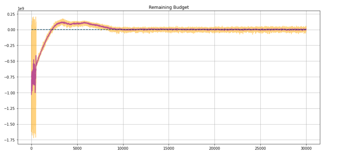
score_history.append(score)Results
Just after some training, our agent performs very well and exhausts almost complete budget.
Reinforcement Learning Libraries in Python
There are plenty of libraries offering implemented RL algorithms like –
- Stable Baselines
- TF Agents
- Keras-RL
- Keras-RL2
- PyQlearning
We will explore a bit on Stable Baselines and how to use them through an example.
Installation
pip install stable-baselines[mpi]Creating Agent with Stable-Baselines
import gym
from stable_baselines import DQN
env = gym.make('MountainCar-v0')
agent = DQN('MlpPolicy', env, learning_rate=1e-3)
agent.learn(total_timesteps=25000)
Now we need an evaluation policy
from stable_baselines.common.evaluation import evaluate_policy

mean_reward, n_steps = evaluate_policy(agent, agent.get_env(), n_eval_episodes=10)

agent.save("DQN_mountain_car_agent") #we can save our agent in the disk

agent = DQN.load("DQN_mountain_car_agent") # or load it
Training the Agent
state = env.reset()

for t in range(5000):
    action, _ = agent.predict(state)
    next_state, reward, done, info = env.step(action)
    state = next_state
    env.render()
This gives us a rough idea, how to use create agents to train in our environment. Since RL is still a heavily research-oriented field, libraries updates fast. Stable baselines has the largest collection of algorithms implemented with additional features. It is suggestive to start with baselines before moving to other libraries.
Challenges in Reinforcement Learning
Reinforcement Learning is very easily prone to errors, local maxima/minima, and debugging it is hard as compared to other machine learning paradigms, it is because RL works on feedback loops and small errors propagate in the whole model. But that’s not it, we have the most crucial part which is assigning the reward function. Agent heavily depends upon the reward as it is the only thing by which it gets feedback. One of the classical problems in RL is exploration vs exploitation. Various novel methods are used to suppress this, for example, DDPG is prone to this issue so authors of TD3 and SAC (both are improvements over DDPG) used two additional networks (TD3) and temperature parameter(SAC) to deal with the exploration vs exploitation problem and many more novel approaches are being worked upon. Even from all the challenges, Deep RL has lots of applications in real life.
Conclusion
This guide provides a comprehensive overview of reinforcement learning (RL), covering fundamental concepts, key elements, practical applications, and popular algorithms. By exploring Markov Decision Processes (MDPs), OpenAI Gym, and deep Q networks (DQN), readers gain a solid understanding of RL principles and techniques. Furthermore, it discusses challenges and introduces libraries like Stable-Baselines for RL implementation. Armed with this knowledge, practitioners can embark on RL projects confidently, equipped with the tools and insights needed to navigate the complexities of training agents in dynamic environments.
The media shown in this article are not owned by Analytics Vidhya and are used at the Author’s discretion.
Frequently Asked Questions?
Q1. What is reinforcement learning (RL)?
A. Reinforcement learning is a type of machine learning where an agent learns to make decisions by interacting with an environment to maximize cumulative rewards.
Q2. What are the key elements fundamental to RL?
A. Key elements include the agent, environment, state, action, reward, and policy, which collectively form the basis of RL systems.
Q3. How does OpenAI Gym facilitate RL training?
A. OpenAI Gym provides a standardized interface for RL environments, allowing users to easily develop and test algorithms across various tasks and scenarios.
Q4. What are some popular algorithms in RL?
A. Popular RL algorithms include Deep Q Network (DQN), Replay Buffer, Critic Network, Actor-Network, and others, which are essential for training agents in complex environments.
Q5. What challenges are associated with RL implementation?
A. Challenges in RL include the exploration-exploitation dilemma, sparse rewards, credit assignment problem, and scalability issues, among others, which necessitate careful consideration during algorithm design and implementation.


