This article was published as a part of the Data Science Blogathon.
Introduction
Generative adversarial networks (GANs), is an algorithmic architecture that consists of two neural networks, which are in competition with each other (thus the “adversarial”) in order to generate new, replicated instances of data that can pass for real data.
The generative approach is an unsupervised learning method in machine learning which involves automatically discovering and learning the patterns or regularities in the given input data in such a way that the model can be used to generate or output new examples that plausibly could have been drawn from the original dataset Their applications include image generation, video generation, and voice generation.
Get ready for an exhilarating experience at DataHack Summit 2023! Join us from August 2nd to 5th at the prestigious NIMHANS Convention Center in vibrant Bengaluru. Brace yourself for mind-blowing workshops, invaluable insights from industry experts, and unparalleled networking with fellow data enthusiasts. Stay ahead, unlock endless possibilities in data science and AI, and seize this incredible opportunity. Mark your calendars, secure your spot, and get ready for an unforgettable journey. Click here for more details!
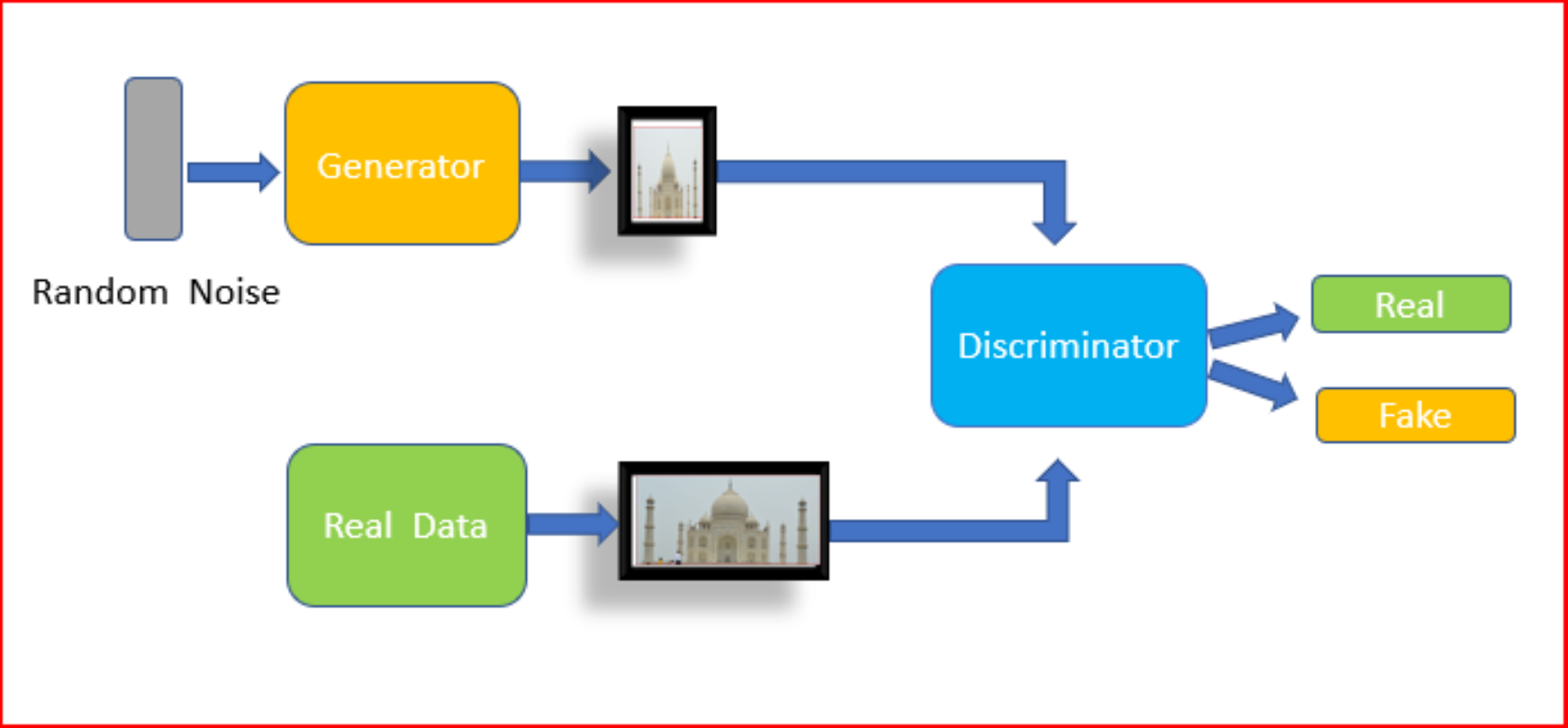
GAN contains Generator and Discriminator
GENERATOR
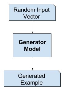
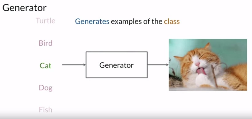
The generator is like the heart. It’s a model that’s used to generate examples and the one that you should be invested in and helping achieve really high performance at the end of the training process. The generator’s goal is to be able to produce synthetic examples from a certain input. So if you trained it from the class of a cat, then the generator will do some computations and output a representation of a cat that looks real.
So ideally, the generator won’t output the same cat at every run, and so to ensure it’s able to produce different examples every single time, the input will be different sets of random values, known as a noise vector. For example, the noise vector can be 1, 2, 5, 1.5, 5, 5, 2. Then this noise vector is fed in as input. After the training, the generator model is used to generate new samples.
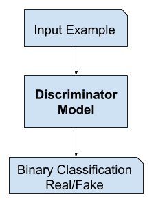
DISCRIMINATOR
source: machinelearningmastery
The discriminator is a type of classifier, the aim is to differentiate between real or fake that is generated data. Classifiers aren’t limited to determining only image classes, You could have video data of any kind, all sorts of different things here. Hence the discriminator is a type of classifier, which learns to model the probability of a given example being real or fake with the help of given input features, like pixel(RGB) values for images. These output probabilities obtained from the discriminator help the generator, so that it can learn to produce better examples over time.
Let’s start
We can generate our own dataset using GAN, we just need a reference dataset for this tutorial, it can be any dataset containing images. I am using google colab for this tutorial
The following packages will be used to implement a basic GAN system in Python/Keras.
import tensorflow as tf
from tensorflow.keras.layers import Input, Reshape, Dropout, Dense
from tensorflow.keras.layers import Flatten, BatchNormalization
from tensorflow.keras.layers import Activation, ZeroPadding2D
from tensorflow.keras.layers import LeakyReLU
from tensorflow.keras.layers import UpSampling2D, Conv2D
from tensorflow.keras.models import Sequential, Model, load_model
from tensorflow.keras.optimizers import Adam
import numpy as np
from PIL import Image
from tqdm import tqdm
import os
import time
import matplotlib.pyplot as plt
The following code mounts your Google drive for use with Google CoLab.
from google.colab import drive
drive.mount('/content/drive')
These are the constants that define how the GANs will be created for this example. The higher the resolution, the more memory that will be needed. Higher resolution will also result in longer run times. For Google CoLab (with GPU) 128×128 resolution is as high as can be used (due to memory). Note that the resolution is specified as a multiple of 32. So GENERATE_RES of 1 is 32, 2 is 64, etc.
To run this you will need training data. The training data can be any collection of images. I suggest using training data from the following two locations. Simply unzip and combine to a common directory. This directory should be uploaded to Google Drive (if you are using CoLab). The constant DATA_PATH defines where these images are stored.
GENERATE_RES = 3 # Generation resolution factor
# (1=32, 2=64, 3=96, 4=128, etc.)
GENERATE_SQUARE = 32 * GENERATE_RES # rows/cols (should be square)
IMAGE_CHANNELS = 3

# Preview image
PREVIEW_ROWS = 4
PREVIEW_COLS = 7
PREVIEW_MARGIN = 16

# Size vector to generate images from
SEED_SIZE = 100

# Configuration
DATA_PATH = '/content/drive/MyDrive/cars/images'
EPOCHS = 50
BATCH_SIZE = 32
BUFFER_SIZE = 60000

print(f"Will generate {GENERATE_SQUARE}px square images.")
#output('Will generate 96px square images.')
Next, we will load and preprocess the images. This can take a while. Google CoLab took around an hour to process. Because of this, we store the processed file as a binary. This way we can simply reload the processed training data and quickly use it. It is most efficient to only perform this operation once. The dimensions of the image are encoded into the filename of the binary file because we need to regenerate it if these change.
training_binary_path = os.path.join(DATA_PATH,
        f'training_data_{GENERATE_SQUARE}_{GENERATE_SQUARE}.npy')

print(f"Looking for file: {training_binary_path}")

if not os.path.isfile(training_binary_path):
  start = time.time()
  print("Loading training images...")

  training_data = []
  faces_path = os.path.join(DATA_PATH)
  for filename in tqdm(os.listdir(faces_path)):
      path = os.path.join(faces_path,filename)
      image = Image.open(path).resize((GENERATE_SQUARE,
            GENERATE_SQUARE),Image.ANTIALIAS)
      training_data.append(np.asarray(image))
  training_data = np.reshape(training_data,(-1,GENERATE_SQUARE,
            GENERATE_SQUARE,IMAGE_CHANNELS))
  training_data = training_data.astype(np.float32)
  training_data = training_data / 127.5 - 1.


  print("Saving training image binary...")
  np.save(training_binary_path,training_data)
  elapsed = time.time()-start
  print (f'Image preprocess time: {hms_string(elapsed)}')
else:
  print("Loading previous training pickle...")
  training_data = np.load(training_binary_path)
We will use a TensorFlow Dataset object to actually hold the images. This allows the data to be quickly shuffled int divided into the appropriate batch sizes for training.
train_dataset = tf.data.Dataset.from_tensor_slices(training_data)
    .shuffle(BUFFER_SIZE).batch(BATCH_SIZE)
Next, we actually build the discriminator and the generator. Both will be trained with the Adam optimizer.
def build_generator(seed_size, channels):
    model = Sequential()

    model.add(Dense(4*4*256,activation="relu",input_dim=seed_size))
    model.add(Reshape((4,4,256)))

    model.add(UpSampling2D())
    model.add(Conv2D(256,kernel_size=3,padding="same"))
    model.add(BatchNormalization(momentum=0.8))
    model.add(Activation("relu"))

    model.add(UpSampling2D())
    model.add(Conv2D(256,kernel_size=3,padding="same"))
    model.add(BatchNormalization(momentum=0.8))
    model.add(Activation("relu"))

    # Output resolution, additional upsampling
    model.add(UpSampling2D())
    model.add(Conv2D(128,kernel_size=3,padding="same"))
    model.add(BatchNormalization(momentum=0.8))
    model.add(Activation("relu"))

    if GENERATE_RES>1:
      model.add(UpSampling2D(size=(GENERATE_RES,GENERATE_RES)))
      model.add(Conv2D(128,kernel_size=3,padding="same"))
      model.add(BatchNormalization(momentum=0.8))
      model.add(Activation("relu"))

    # Final CNN layer
    model.add(Conv2D(channels,kernel_size=3,padding="same"))
    model.add(Activation("tanh"))

    return model


def build_discriminator(image_shape):
    model = Sequential()

    model.add(Conv2D(32, kernel_size=3, strides=2, input_shape=image_shape,
                     padding="same"))
    model.add(LeakyReLU(alpha=0.2))

    model.add(Dropout(0.25))
    model.add(Conv2D(64, kernel_size=3, strides=2, padding="same"))
    model.add(ZeroPadding2D(padding=((0,1),(0,1))))
    model.add(BatchNormalization(momentum=0.8))
    model.add(LeakyReLU(alpha=0.2))

    model.add(Dropout(0.25))
    model.add(Conv2D(128, kernel_size=3, strides=2, padding="same"))
    model.add(BatchNormalization(momentum=0.8))
    model.add(LeakyReLU(alpha=0.2))

    model.add(Dropout(0.25))
    model.add(Conv2D(256, kernel_size=3, strides=1, padding="same"))
    model.add(BatchNormalization(momentum=0.8))
    model.add(LeakyReLU(alpha=0.2))

    model.add(Dropout(0.25))
    model.add(Conv2D(512, kernel_size=3, strides=1, padding="same"))
    model.add(BatchNormalization(momentum=0.8))
    model.add(LeakyReLU(alpha=0.2))

    model.add(Dropout(0.25))
    model.add(Flatten())
    model.add(Dense(1, activation='sigmoid'))

    return model
As we progress through training images will be produced to show the progress. These images will contain a number of rendered image data that show how good the generator has become.
def save_images(cnt,noise):
  image_array = np.full((
      PREVIEW_MARGIN + (PREVIEW_ROWS * (GENERATE_SQUARE+PREVIEW_MARGIN)),
      PREVIEW_MARGIN + (PREVIEW_COLS * (GENERATE_SQUARE+PREVIEW_MARGIN)), 3),
      255, dtype=np.uint8)

  generated_images = generator.predict(noise)

  generated_images = 0.5 * generated_images + 0.5

  image_count = 0
  for row in range(PREVIEW_ROWS):
      for col in range(PREVIEW_COLS):
        r = row * (GENERATE_SQUARE+16) + PREVIEW_MARGIN
        c = col * (GENERATE_SQUARE+16) + PREVIEW_MARGIN
        image_array[r:r+GENERATE_SQUARE,c:c+GENERATE_SQUARE]
            = generated_images[image_count] * 255
        image_count += 1


  output_path = os.path.join(DATA_PATH,'output')
  if not os.path.exists(output_path):
    os.makedirs(output_path)

  filename = os.path.join(output_path,f"train-{cnt}.png")
  im = Image.fromarray(image_array)
  im.save(filename)
generator = build_generator(SEED_SIZE, IMAGE_CHANNELS)

noise = tf.random.normal([1, SEED_SIZE])
generated_image = generator(noise, training=False)

plt.imshow(generated_image[0, :, :, 0])
image_shape = (GENERATE_SQUARE,GENERATE_SQUARE,IMAGE_CHANNELS)

discriminator = build_discriminator(image_shape)
decision = discriminator(generated_image)
print (decision)
This will give tensors.
Loss functions must be developed that allow the generator and discriminator to be trained in an adversarial way. Because these two neural networks are being trained independently they must be trained in two separate passes. This requires two separate loss functions and also two separate updates to the gradients.
cross_entropy = tf.keras.losses.BinaryCrossentropy()

def discriminator_loss(real_output, fake_output):
    real_loss = cross_entropy(tf.ones_like(real_output), real_output)
    fake_loss = cross_entropy(tf.zeros_like(fake_output), fake_output)
    total_loss = real_loss + fake_loss
    return total_loss

def generator_loss(fake_output):
    return cross_entropy(tf.ones_like(fake_output), fake_output)
Both the generator and discriminator use Adam and the same learning rate and momentum. This does not need to be the case. If you use a GENERATE_RES greater than 3 you may need to tune these learning rates, as well as other training and hyperparameters.
generator_optimizer = tf.keras.optimizers.Adam(1.5e-4,0.5)
discriminator_optimizer = tf.keras.optimizers.Adam(1.5e-4,0.5)
The following function is where most of the training takes place for both the discriminator and the generator. This function was based on the GAN provided by the TensorFlow Keras examples documentation. The first thing you should notice about this function is that it is annotated with the tf.function annotation. This causes the function to be precompiled and improves performance.
@tf.function
def train_step(images):
  seed = tf.random.normal([BATCH_SIZE, SEED_SIZE])

  with tf.GradientTape() as gen_tape, tf.GradientTape() as disc_tape:
    generated_images = generator(seed, training=True)

    real_output = discriminator(images, training=True)
    fake_output = discriminator(generated_images, training=True)

    gen_loss = generator_loss(fake_output)
    disc_loss = discriminator_loss(real_output, fake_output)


    gradients_of_generator = gen_tape.gradient(
        gen_loss, generator.trainable_variables)
    gradients_of_discriminator = disc_tape.gradient(
        disc_loss, discriminator.trainable_variables)

    generator_optimizer.apply_gradients(zip(
        gradients_of_generator, generator.trainable_variables))
    discriminator_optimizer.apply_gradients(zip(
        gradients_of_discriminator,
        discriminator.trainable_variables))
  return gen_loss,disc_loss
Start the training.
def train(dataset, epochs):
  fixed_seed = np.random.normal(0, 1, (PREVIEW_ROWS * PREVIEW_COLS,
                                       SEED_SIZE))
  start = time.time()

  for epoch in range(epochs):
    epoch_start = time.time()

    gen_loss_list = []
    disc_loss_list = []

    for image_batch in dataset:
      t = train_step(image_batch)
      gen_loss_list.append(t[0])
      disc_loss_list.append(t[1])

    g_loss = sum(gen_loss_list) / len(gen_loss_list)
    d_loss = sum(disc_loss_list) / len(disc_loss_list)

    epoch_elapsed = time.time()-epoch_start
    print (f'Epoch {epoch+1}, gen loss={g_loss},disc loss={d_loss},'
           ' {hms_string(epoch_elapsed)}')
    save_images(epoch,fixed_seed)

  elapsed = time.time()-start
  print (f'Training time: {hms_string(elapsed)}')
train(train_dataset, EPOCHS)
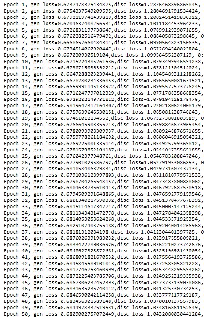
The output after 80+ epochs is impressive. Try it out for yourself.
The link for the complete code – https://github.com/BakingBrains/Generation_of_Data_using_GAN
Linkedin: www.linkedin.com/in/syed-abdul-gaffar-shakhadri-a44111187
The media shown in this article on GAN are not owned by Analytics Vidhya and is used at the Author’s discretion.
Before you go, check this out! Here’s an exclusive recommendation just for you. Level up your data game at the DataHack Summit 2023, where we’ve curated mind-blowing workshops that will revolutionize your skills. From ‘Applied Machine Learning with Generative AI‘, ‘The Art of Productionizing Machine Learning Model‘ and ‘Mastering LLMs: Training, Fine-tuning, and Best Practices‘, these workshops are your golden ticket to unlocking immense value. Dive into hands-on experiences, gain practical skills, and connect with industry leaders. This is your chance to open doors to exciting career opportunities. Secure your spot now for the highly anticipated DataHack Summit 2023.
Syed Abdul Gaffar Shakhadri
03 Jul, 2023
I am an enthusiastic AI developer, I love playing with different problems and building solutions.


When trying to load images I get ValueError: Cannot load file containing pickled data when allow_pickle=False Seems like a lot of people are having this problem but what might be the solution in this case? Thanks, very interesting work!
please whats the benchmark for this?