Portfolio Optimization using MPT in Python

Introduction

In this article, we shall learn the concepts of portfolio management and implement the same by using python libraries.

The article is divided into three parts in order to cover the fundamental aspects of the portfolio management as shown below:

1. Returns on an Asset & Portfolio

2. Risk associated with an Asset & Portfolio

3. Modern Portfolio Theory: Finding the Optimal Portfolio

Returns on an Asset & Portfolio

Before we dive into the computation of the returns on an asset and portfolio, let us briefly visit the definition of portfolio and returns. 

Portfolio: A portfolio is a collection of financial instruments like stocks, bonds, commodities, cash and cash equivalents , as well as their fund counterparts. [Investopedia]

In this article, we will have our portfolio containing 4 assets (“Equities-focused portfolio“): the shares of Apple Inc. , Nike (NKC), Google and Amazon . The preview of our data is shown below:

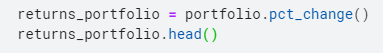
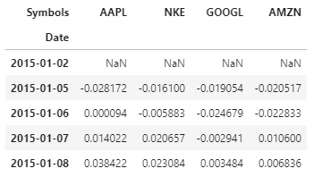
Returns: It refers to the gain or loss on our asset/portfolio over a fixed time frame. In this analysis, we make a return as the percentage change in the closing price of the asset over the previous day’s closing price. We will compute the returns using .pct_change() function in python.

Below is shown the python code to do the same and the top 5 rows (head) of the returns

Note: the first row is Null if there doesn’t exist a row prior to that to facilitate the computation of percentage change.

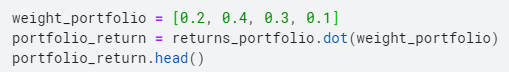
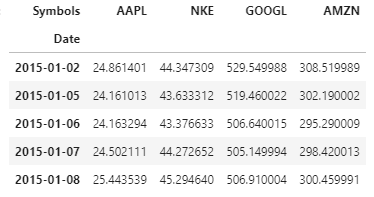
Return of a portfolio is defined as the weighted sum of the returns of the assets in the portfolio.

In order to demonstrate how to compute portfolio return in python, let us initialize the weights randomly (which we will later optimize). The portfolio return is computed as shown in the code below and the head of the portfolio returns is shown as well:

We have seen how to calculate the returns, now lets shift our focus on another concept : Risk

The Risk Associated with Asset & Portfolio

The method to compute the risk of a portfolio is written below and subsequently we explain and give the mathematical formulation for each of the step :

• Calculate the covariance matrix on the returns data
• Annualize the covariance by multiplying by 252
• Compute the portfolio variance by multiplying it with weight vectors
• Compute the square root of the variance calculated above to get the standard deviation. This standard deviation is called as the Volatility of the portfolio

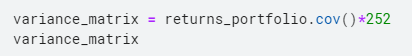
The formula to compute the covariance and annualizing it is :

                                                 covariance = returns.cov()*252

since there are 252 trading days, we multiply the covariance by 252 in order to annualize it.

The portfolio variance , to be calculated in step3 above, depends on the weights of the assets in the portfolio and is defined as :

where, 

• Cov_portfolio is the covariance matrix of the portfolio
• weights is the vector of weights allocated to each asset in the portfolio

Below is shown the approach to compute the asset risk in python.

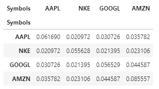
 As explained above we multiple the covariance matrix with 252 as there are 252 trading days in a year.

The diagonal elements of the variance_matrix represent the variance of each asset, while the off-diagonal terms represent the covariance between the two assets, eg: (1,2) element represents the covariance between Nike and Apple.

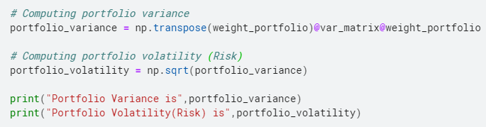
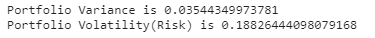
The code to compute the portfolio Risk in python, the method of which we saw above, is as shown:

Now, the task for us is to optimize the weights. Why? So that we can maximize our return or minimize our risk – and that we do by using the Modern Portfolio Theory!

Modern Portfolio Theory

Modern portfolio theory argues that an investment’s risk and return characteristics should not be viewed alone, but should be evaluated by how the investment affects the overall portfolio’s risk and return. MPT shows that an investor can construct a portfolio of multiple assets that will maximize returns for a given level of risk. Likewise, given a desired level of expected return, an investor can construct a portfolio with the lowest possible risk. Based on statistical measures such as variance and correlation, an individual investor’s performance is less important than how it impacts the entire portfolio [Investopedia]

This theory is summarized in the figure below. We find the frontier as shown below and either maximize the Expected Returns for Risk level or minimize Risk for a given Expected Return level.

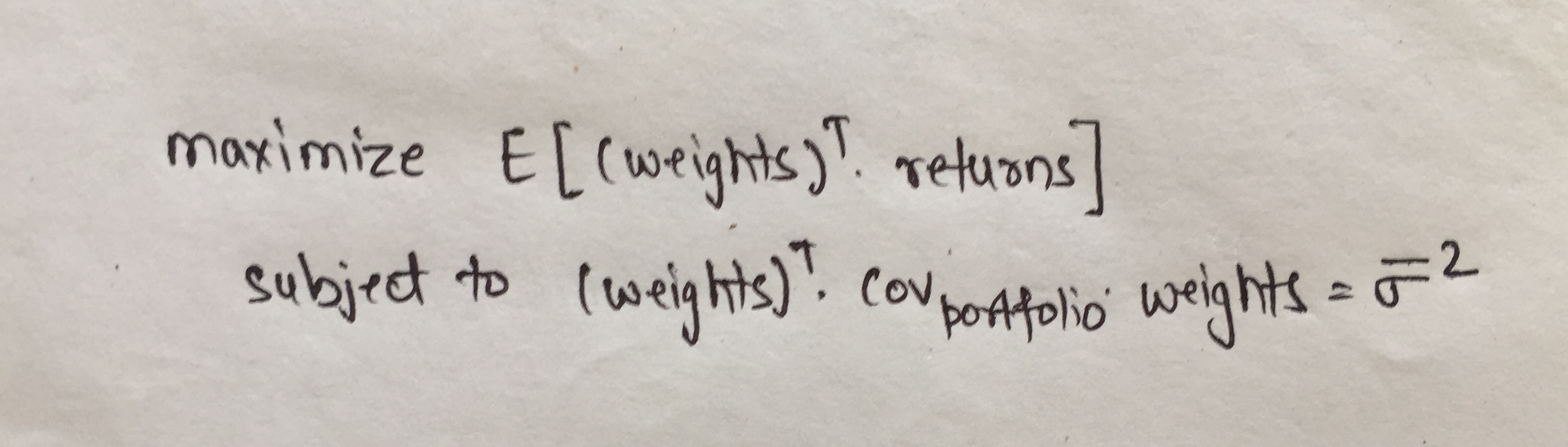
Our goal is to choose the weights for each asset in our portfolio such that we maximize the expected return given a level of risk .

Mathematically, the objective function can be define as shown below:

Another way to look at the Efficient Frontier and the objective function is that we can minimize the risk given that the Expected return is at least greater than is given value. Mathematically this objective function can be written as:

 

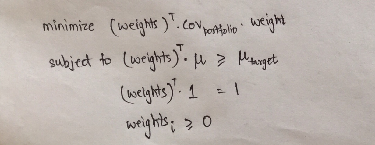
the first line represents that the objective is to minimize the portfolio variance , i.e in turn the portfolio volatility and therefore minimizing the risk.

The subject to constraints implies that the returns have to be greater than a particular target return, all the weights should sum to 1 and weights should not be negative.

Now, that we know the concept, let’s go to the hands-on part now!

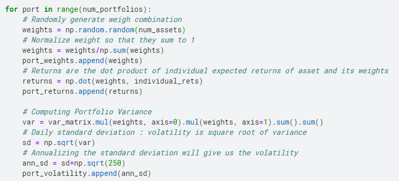
Firstly, we create the efficient frontier by running a loop. In each loop, we consider a randomly allocated different set of weights for the assets in our portfolio and calculate the return and volatility for that combination of weights.

For this purpose we create 3 empty lists , one for storing the returns , another for storing the volatility and the last one for storing the portfolio weights.

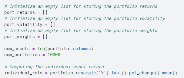
Once we have created the lists, we randomly generate the weights for our assets repeatedly , then normalized the weight to sum to 1. We then compute the returns in the same manner as we calculated earlier. Subsequently, we compute the portfolio variance and then we take the square root and then annualize it to get the volatility, the measure of risk for our portfolio.

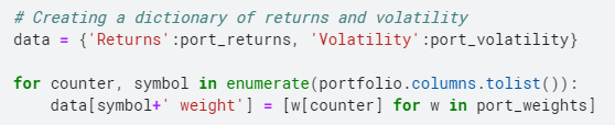
We now aggregate the data into a dictionary and then create a dataframe to see the weight combination for the assets and the corresponding returns and volatility that they generate.

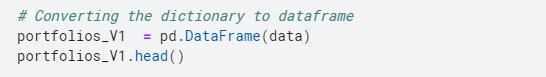
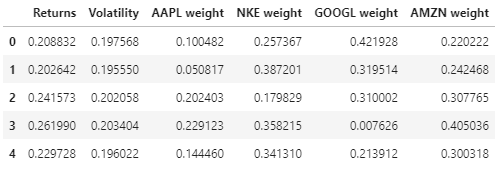
Here is the preview of the data of portfolio returns, volatility and weights.

Now we have everything with us to enter into the final lap of this race and find the optimal set of weights!

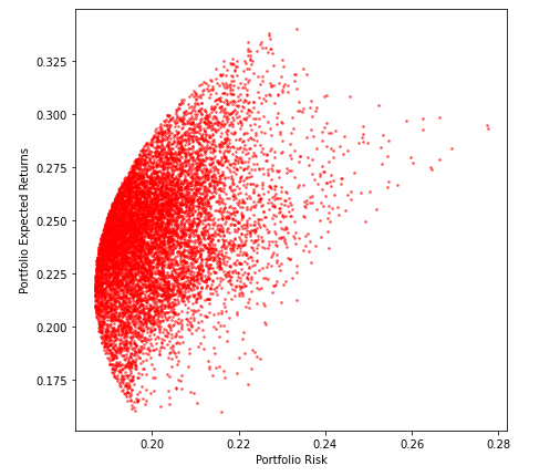
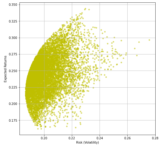
We plot Volatility against the returns that we compute above, this will give us the Efficient Frontier that we wanted to create at the beginning of this article.

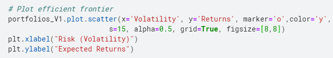
And here we go!!

Now that we have with us the Efficient Frontier, let’s find the optimal weights.

We can optimize the using multiple methods as written below:

• Portfolio with minimum Volatility (Risk)
• Optimal Portfolio (Maximum Sharpe Ratio)
• Maximum returns at a risk level; Minimum Risk at an Expected Return Level; Portfolio with highest Sortino Ratio

In this article I will optimize via the first two approaches. In the third segment the ‘Maximum returns at a risk level’ and ‘Minimum Risk at a Expected Return Level’ are pretty straight forward while the one based on Sortino Ratio is similar to Sharpe Ratio

1. Minimum Volatility

To find the minimum volatility combination, we select the row in our dataframe which corresponds to the minimum variance and we find that row using the .idxmin() function. The code to do the same is shown below:

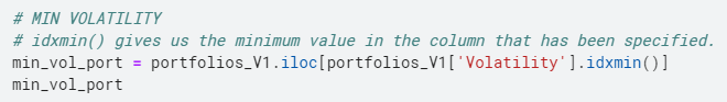
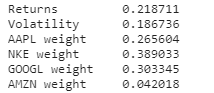
The weights that we get from this are:

Now, find out where will the minimum volatility point lies on the above curve ? The answer is shown at the end! Don’t cheat though!

2. Highest Sharpe Ratio

The Sharpe-ratio is the average return earned in excess of the risk-free rate per unit of volatility or total risk. The formula used to calculate Sharpe-ratio is given below:

                                                            Sharpe Ratio = (R_p – R_f)/ SD_p

where,

• R_p is the return of portfolio
• R_f is the risk free rate
• SD_p is the standard deviation of the portfolio’s returns

The code to compute the most optimal portfolio, i.e the portfolio with the highest Sharpe Ratio is shown below:

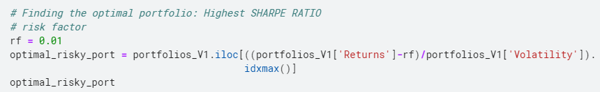
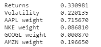
The weights of the portfolio giving the highest Sharpe Ratio are shown below:

Find out where will the highest Sharpe Ratio point lies on the above curve ? The answer is shown below! Again, Don’t cheat!

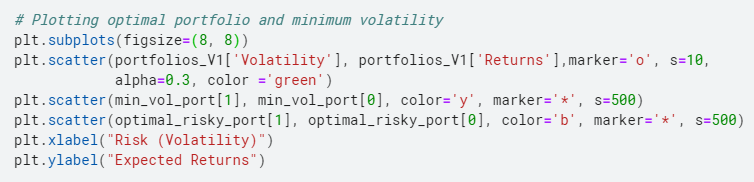
As promised here is the answer to the above two question!

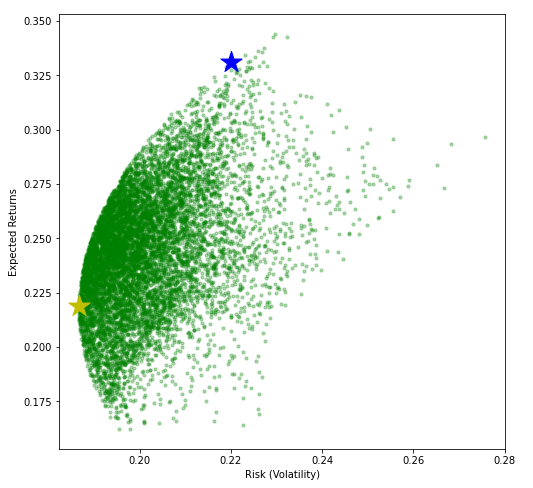
The blue star corresponds to the highest Sharpe ratio point and the yellow star corresponds to the minimum volatility point.

Now, before ending this article I encourage you to find the Maximum returns at a risk level’ and ‘Minimum Risk at an Expected Return Level’ portfolio and mark them on the graph above.

Apart from using the Sharpe Ratio, we can optimize the portfolio using the Sortino Ratio as well.

Giving a brief about it:

The Sortino ratio is a variation of the Sharpe Ratio that differentiates harmful volatility from total overall volatility by using the asset’s standard deviation of negative portfolio returns—downside deviation—instead of the total standard deviation of portfolio returns. The Sortino ratio takes an asset or portfolio’s return and subtracts the risk-free rate, and then divides that amount by the asset’s downside deviation. [Investopedia]

                                                      Sortino Ratio = (R_p – r_f)/ SDd

where,

• R_p is the return of the portfolio
• r_f is the risk free rate
• SDd is the standard deviation of the downside

In case you have any issue implementing or understanding the 3 optimization methods I described above, do write to me at the [email protected] | [email protected] | or reach out at LinkedIn at https://www.linkedin.com/in/parth-tyagi-4b867452/

Note about the author: Parth Tyagi is currently pursuing PGDBA from IIM Calcutta, IIT Kharagpur & Indian Statistical Institute-Kolkata and has completed the B.Tech from IIT Delhi. He has ~4 years of work experience in Advanced Analytics.