Introduction
If you are an aspiring Data Analyst / Data Scientist, am sure you know that Data Wrangling is one of the most crucial steps for any Data Science or Machine Learning project and it’s the longest too.
Python programming language has a powerful and popular package ‘Pandas’ built on top of Numpy which has the implementation of many data objects and data operations. Pandas is one of the most famous data science tools and it’s definitely a game-changer for cleaning, manipulating, and analyzing data.
In this article, we will explore two of the most important data structures of pandas:
- 1. Series
- 2. DataFrame
We will also conduct hands-on Exploratory Data Analysis on an intriguing dataset on movies, learning some of the most useful operations and functionalities that pandas offer by directly analyzing real data, accessible to beginners as well.
Learning Objectives
- Recognize data wrangling’s pivotal role in data science and machine learning workflows.
- Appreciate Pandas’ utility in streamlining data cleaning, manipulation, and analysis.
- Differentiate between Pandas’ Series and DataFrame structures.
- Understand the one-dimensional and two-dimensional representations of Series and DataFrame.
- Learn to create Series and DataFrame objects from various data sources like lists, arrays, dictionaries, and files.
This article was published as a part of the Data Science Blogathon.
Table of contents
- Introduction
- Why Pandas?
- Series
- How to Create a Series?
- DataFrame
- Create a Dataframe from Series object
- Create DataFrame from a dictionary object
- Create a dataframe by importing data from File
- Read Data
- View Data
- Understand Basic Information About the Data
- Data Selection – Indexing and Slicing
- Data Selection – Based on Conditional Filtering
- Groupby Operation
- Sorting Operation
- Dealing with Missing Values
- Dropping Columns and Null Values
- Apply( ) Function
- Conclusion
- Frequently Asked Questions
Why Pandas?
Pandas provide tools for reading and writing data into data structures and files. It also provides powerful aggregation functions to manipulate data.
Pandas provide extended data structures to hold different types of labeled and relational data. This makes python highly flexible and extremely useful for data cleaning and data manipulation.
Pandas is highly flexible and provides functions for performing operations like merging, reshaping, joining, and concatenating data.
Let’s first look at the two most used data structures provided by Pandas.
Series
A Series resembles a 1-D array or a single column of a 2D array or matrix, akin to a column in an Excel sheet. It comprises data values linked to specific labels, with each row having distinct index values. These indexes are automatically assigned upon Series creation, but we can also define them explicitly.
Let’s dive in, create and explore Series by actually writing code in a Jupyter notebook.
Open your Jupyter notebook and follow along!
The Jupyter notebook with the code for this article can be accessed here.
How to Create a Series?
A series object can be created from either a list or an array of values or from a dictionary with key-value pairs.
pd.Series( ) is the method used to create Series. It can take a list, array, or dictionary as a parameter.
Create Series from List
Let’s create a Series using a list of values
Python Code:
# importing pandas library
import pandas as pd

s1 = pd.Series([10,20,30,40,50])
print("The series values are:", s1.values)
print("The index values are:", s1.index.values)
Here, the indexes are generated by default, but we can also define custom indexes at the time of Series creation.
Below is a Series of ‘Marks’ and associated ‘Subjects’. The list of subjects is set as a row index.
s2 = pd.Series([80,93,78,85,97], index=['English','Science','Social','Tamil','Maths'])
print("The Marks obtained by student are", s2)

The Marks obtained by student are Subject
English    80
Science    93
Social     78
Tamil      85
Maths      97
Name: Student Marks, dtype: int64
Indexing and Slicing operation in Series
Data retrieval and manipulation are the most essential operations that we perform during data analysis. Data stored in a Series can be retrieved using slicing operation by square brackets [ ]
# slicing using default integer index
s1[1:4]

1    20
2    30
3    40
dtype: int64

# Slicing using string index

s2[‘Tamil’]

85
Create Series from Dictionary
A dictionary is a core Python data structure that stores data as a set of Key-Value pairs. A Series is also similar to a dictionary in a way that it maps given indexes to a set of values.
I have a dictionary that stores data about fruits and their prices. Let’s see how to create Series from this dictionary. We can also look at data types.
dict_fruits = { 'Orange':80,
          'Apples':210,
          'Bananas':50,
         'Grapes':90,
         'Watermelon':70}
Let’s convert ‘dict_fruits’ to a Series
# Lets convert this dictionary into a series
fruits = pd.Series(dict_fruits)

print("Fruits and pricesn", fruits)

Fruits and prices
 Orange         80
Apples        210
Bananas        50
Grapes         90
Watermelon     70
dtype: int64
Data from this series can be retrieved as below:
# Slice the series and retrieve price of Grapes

print("The price per kg of grapes is:", fruits['Grapes'])

The price per kg of grapes is: 90
DataFrame
The next important data structure in pandas is the most widely used ‘DataFrame’.
A Pandas DataFrame can be thought of as a multi-dimensional table or a table of data in an excel file. It is a multi-dimensional table structure essentially made up of a collection of Series. It helps us store tabular data where each row is an observation and the columns represent variables.
pd.DataFrame( ) is the function used to create a dataframe.
A DataFrame can be created in multiple ways. Let’s look at each one of them:
Create a Dataframe from Series object
A dataframe can be created by passing a series (or multiple) into the DataFrame creation method. The columns can be named using the optional input parameter ‘columns’
Let’s create a Dataframe using the Series we created in the above step:
df_marks = pd.DataFrame(s2, columns=['Student1'])
print("The dataframe created from series isn",df_marks)

The dataframe created from series is
          Student1
English        80
Science        93
Social         78
Tamil          85
Maths          97
Create DataFrame from a dictionary object
Let’s say we have 2 series of heights and weights of a set of persons and we want to put it together in a table.
# Create Height series (in feet)
height = pd.Series([5.3, 6.2,5.8,5.0,5.5], index=['Person 1','Person 2','Person 3','Person 4','Person 5'])
# Create Weight Series (in kgs)
weight = pd.Series([65,89,75,60,59], index=['Person 1','Person 2','Person 3','Person 4','Person 5'])
We will create a dictionary using both ‘height’ and ‘weight’ Series, and finally, create a dataframe using pd.DataFrame( ) method.
# Create dataframe
df_person = pd.DataFrame({'height': height, 'weight': weight})
print("The Person table details are:n", df_person)

The Person table details are:
           height  weight
Person 1     5.3      65
Person 2     6.2      89
Person 3     5.8      75
Person 4     5.0      60
Person 5     5.5      59
Create a dataframe by importing data from File
Pandas is extremely useful and comes in handy when we want to load data from various file formats like CSV, Excel, JSON, etc.
Here are few methods to read data into dataframe from other file objects
- read_table( )
- read_csv( )
- read_html( )
- read_json( )
- read_pickle( )
For the purpose of this article, we will consider only reading data from the CSV file.
Data Analysis of IMDB movies data
As we have a basic understanding of the different data structures in Pandas, let’s explore the fun and interesting ‘IMDB-movies-dataset’ and get our hands dirty by performing practical data analysis on real data.
It is an open-source dataset and you can download it from this link.
What’s more fun than performing hands-on data analysis?
So put on your hats as a Data Analyst/ Data Scientist and let’s GET.SET.GO
We will read the data from the .csv file and perform the following basic operations on movies data
- Read data
- View the data
- Understand some basic information about the data
- Data Selection – Indexing and Slicing data
- Data Selection – Based on Conditional filtering
- Groupby operations
- Sorting operation
- Dealing with missing values
- Dropping columns and null values
- Apply( ) functions
Read Data
Load data from CSV file.
# Read data from .csv file
data = pd.read_csv('IMDB-Movie-Data.csv')

# Read data with specified explicit index.
# We will use this later in our analysis
data_indexed = pd.read_csv('IMDB-Movie-Data.csv', index_col="Title")
View Data
Let’s do a quick preview of the data by using head( ) and tail( ) methods
head( )
- Returns the top 5 rows in the dataset by default
- It can also take the number of rows to be viewed as a parameter
tail( )
- Returns the bottom 5 rows in the dataset by default
- It can also take the number of rows as an optional parameter
# Preview top 5 rows using head()
data.head()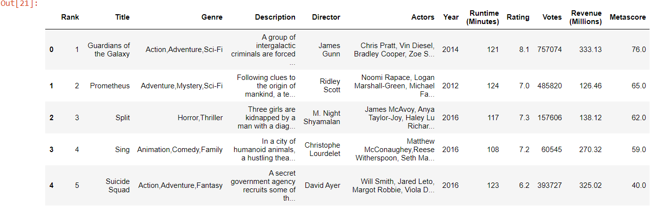
Understand Basic Information About the Data
Pandas provide many functions to understand the shape, number of columns, indexes, and other information about the dataframe.
- info( ) is one of my favorite methods that gives all necessary information about different columns in a dataframe.
#Lets first understand the basic information about this data
data.info()

<class 'pandas.core.frame.DataFrame'>
RangeIndex: 1000 entries, 0 to 999
Data columns (total 12 columns):
 #   Column              Non-Null Count  Dtype
---  ------              --------------  -----
 0   Rank                1000 non-null   int64
 1   Title               1000 non-null   object
 2   Genre               1000 non-null   object
 3   Description         1000 non-null   object
 4   Director            1000 non-null   object
 5   Actors              1000 non-null   object
 6   Year                1000 non-null   int64
 7   Runtime (Minutes)   1000 non-null   int64
 8   Rating              1000 non-null   float64
 9   Votes               1000 non-null   int64
 10  Revenue (Millions)  872 non-null    float64
 11  Metascore           936 non-null    float64
dtypes: float64(3), int64(4), object(5)
memory usage: 93.9+ KB- shape can be used to get the shape of dataframe
- columns gives us the list of columns in the dataframe
data.shape
(1000, 12)
This function tells us that there are 1000 rows and 12 columns in the dataset
- describe( ) method gives the basic statistical summaries of all numerical attributes in the dataframe.
data.describe()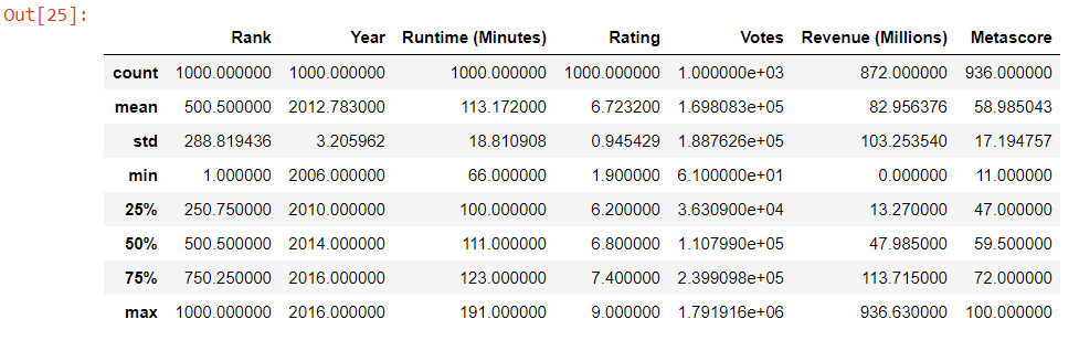
Some Insights from the Description Table
- The min and max values in ‘Year’ depict the minimum and maximum release years. We can see that the dataset contains movies from 2006 to 2016.
- The average rating for the movies in this dataset is about 6.7 and the minimum rating is 1.9 and the maximum rating is 9.0
- The maximum revenue earned by a movie is 936.6 million
Data Selection – Indexing and Slicing
Extract Data Using Columns
Extracting data from a dataframe is similar to Series. Here the column label is used to extract data from the columns.
Let’s quickly extract ‘Genre’ data from the dataframe
# Extract data as series
genre = data['Genre']
This operation will retrieve all the data from the ‘Genre’ column as Series. If we want to retrieve this data as a dataframe, then indexing must be done using double square brackets as below:
# Extract data as dataframe
data[['Genre']]
If we want to extract multiple columns from the data, simply add the column names to the list.
some_cols = data[['Title','Genre','Actors','Director','Rating']]Extract Data Using Rows
loc and iloc are two functions that can be used to slice data from specific row indexes.
loc – locates the rows by name
- loc performs slicing based explicit index.
- It takes string indexes to retrieve data from specified rows
iloc – locates the rows by integer index
- iloc performs slicing based on Python’s default numerical index.
In the beginning, when we read the data, we created a dataframe with ‘Title’ as the string index.
We will use the loc function to index and slice that dataframe using the specified ‘Title’.
data_indexed.loc[['Suicide Squad']][['Genre','Actors','Director','Rating','Revenue (Millions)']]Here, iloc is used to slice data using integer indexes.
data.iloc[10:15][['Title','Rating','Revenue (Millions)']]Data Selection – Based on Conditional Filtering
Pandas also enable retrieving data from dataframe based on conditional filters.
What if we want to pick only movies that are released from 2010 to 2016, have a rating of less than 6.0 but topped in terms of revenue?
It’s very simple and can be retrieved in a single line of code…
data[((data['Year'] >= 2010) & (data['Year'] <= 2016))
      & (data['Rating'] < 6.0)
      & (data['Revenue (Millions)'] > data['Revenue (Millions)'].quantile(0.95))]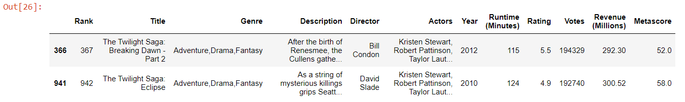
‘The Twilight Saga: Breaking Dawn – Part 2′ and ‘The Twilight Saga: Eclipse’ are the movies that topped in the box office, despite having lower ratings.
Groupby Operation
Data can be grouped and operations can be performed on top of grouped data by using the groupby( ) method. This comes in handy when we want to apply aggregations and functions on top of grouped data.
data.groupby('Director')[['Rating']].mean().head()| Director | Rating |
|---|---|
| Aamir Khan | 8.5 |
| Abdellatif Kechiche | 7.8 |
| Adam Leon | 6.5 |
| Adam McKay | 7.0 |
| Adam Shankman | 6.3 |
Director Rating Aamir Khan 8.5 Abdellatif Kechiche 7.8 Adam Leon 6.5 Adam McKay 7.0 Adam Shankman 6.3.
Sorting Operation
Sorting is yet another pandas operation that is heavily used in data analysis projects.
sort_values( ) method is used to perform sorting operation on a column or a list of multiple columns
In the above example, where we have listed the average rating for each ‘Director’, if we want to sort them from highly rated to lowest, we can perform the sorting operation.
data.groupby('Director')[['Rating']].mean().sort_values(['Rating'], ascending=False).head()| Director | Rating |
|---|---|
| Nitesh Tiwari | 8.80 |
| Christopher Nolan | 8.68 |
| Makoto Shinkai | 8.60 |
| Olivier Nakache | 8.60 |
| Florian Henckel von Donnersmarck | 8.50 |
Director Rating Nitesh Tiwari 8.80 Christopher Nolan 8.68 Makoto Shinkai 8.60 Olivier Nakache 8.60 Florian Henckel von Donnersmarck 8.50.
We can see that Director ‘Nitesh Tiwari’ has the highest average rating in this dataset.
Dealing with Missing Values
Pandas has isnull( ) for detecting null values (nan) in a dataframe. Let’s see how to use these methods.
# To check null values row-wise
data.isnull().sum()

Rank                    0
Title                   0
Genre                   0
Description             0
Director                0
Actors                  0
Year                    0
Runtime (Minutes)       0
Rating                  0
Votes                   0
Revenue (Millions)    128
Metascore              64
dtype: int64
Here we know that ‘Revenue (Millions)’ and ‘Metascore’ are two columns where there are null values.
As we have seen null values in data, we can either choose to drop those or impute these values.
Dropping Columns and Null Values
Dropping columns/rows is yet another operation that is most important for data analysis.
drop( ) function can be used to drop rows or columns based on condition.
# Use drop function to drop columns
data.drop('Metascore', axis=1).head()
Using the above code, the ‘Metascore’ column is dropped completely from data. Here axis= 1 specifies that column is to be dropped. These changes will not take place in actual data unless we specify inplace=True as a parameter in the drop( ) function.
We can also drop rows/ columns with null values by using dropna( ) function.
# Drops all rows containing missing data
data.dropna()

# Drop all columns containing missing data
data.dropna(axis=1)

data.dropna(axis=0, thresh=6)
In the above snippet, we are using thresh parameter to specify the minimum number of non-null values for the column/row to be held without dropping.
In our movies data, we know that there are some records where the Revenue is null.We can impute these null values with mean Revenue (Millions).
fillna( ) –> function used to fill null values with specified values.
revenue_mean = data_indexed['Revenue (Millions)'].mean()
print("The mean revenue is: ", revenue_mean)

The mean revenue is:  82.95637614678897

# We can fill the null values with this mean revenue
data_indexed['Revenue (Millions)'].fillna(revenue_mean, inplace=True)
Now, if we check the dataframe, there won’t be any null values in the Revenue column.
Apply( ) Function
The apply( ) function comes in handy when we want to apply any function to the dataset. It returns a value after passing each row of the dataframe to some function. The function can be built-in or user-defined.
For example, if we want to classify the movies based on their ratings, we can define a function to do so and then apply the function to the dataframe as shown below.
I will write a function that will classify movies into groups based on rating.
# Classify movies based on ratings
def rating_group(rating):
    if rating >= 7.5:
        return 'Good'
    elif rating >= 6.0:
        return 'Average'
    else:
        return 'Bad'
Now, I will apply this function to our actual dataframe and the ‘Rating_category’ will be computed for each row.
# Lets apply this function on our movies data
# creating a new variable in the dataset to hold the rating category
data['Rating_category'] = data['Rating'].apply(rating_group)
Here is the resultant data after applying the rating_group( ) function.
data[['Title','Director','Rating','Rating_category']].head(5)| Title | Director | Rating | Rating_category | |
|---|---|---|---|---|
| 0 | Guardians of the Galaxy | James Gunn | 8.1 | Good |
| 1 | Prometheus | Ridley Scott | 7.0 | Average |
| 2 | Split | M. Night Shyamalan | 7.3 | Average |
| 3 | Sing | Christophe Lourdelet | 7.2 | Average |
| 4 | Suicide Squad | David Ayer | 6.2 | Average |
We learned about most of the important operations in Pandas that are needed for data processing and manipulation. And it was great fun analyzing the IMBD movies data.
If you would like to delve deep into some of these operations, please have a look at this article’s Jupyter notebook from my Github.
Conclusion
In conclusion, this tutorial has provided a comprehensive step-by-step guide to data analysis using Python pandas with the IMDb dataset. By leveraging pandas functions, we’ve demonstrated how to manipulate, clean, and analyze data efficiently.
Armed with this knowledge, you can harness the power of pandas to tackle diverse datasets and extract valuable insights. With its intuitive API and extensive functionality, pandas remains an indispensable tool for data analysis tasks. Whether you’re a beginner or a seasoned practitioner, this tutorial serves as a valuable resource for mastering pandas and advancing your data analysis skills.
Frequently Asked Questions
Q1. Can we use pandas library for data visualization?
A. Yes, pandas can be used for basic data visualization. It integrates with Matplotlib for plotting graphs directly from DataFrames and Series, offering a convenient way to visualize data.
Q2. How does sql compare to pandas?
A. SQL is designed for managing and querying data in databases, focusing on data manipulation and retrieval. Pandas, on the other hand, is a Python library for data analysis and manipulation, offering in-memory data manipulation capabilities. While SQL operates on data stored in databases, pandas works with data in memory, providing more flexible data manipulation and analysis features.
Q3. Is pandas enough for data analysis?
A. Pandas is powerful for data manipulation and analysis, especially for structured data, offering extensive functionality for data cleaning, transformation, and analysis. However, for advanced statistical analysis, machine learning, or big data processing, integrating pandas with libraries like NumPy, SciPy, scikit-learn, or PySpark might be necessary.
The media shown in this article are not owned by Analytics Vidhya and is used at the Author’s discretion.


Just read this article and I must say it's been a huge help for me to understand pandas better. I've been struggling with data analysis for weeks now, but your guide has clarified a lot of concepts for me. Thanks for the effort you put into writing such an informative post!