Image Segmentation With Felzenszwalb’s Algorithm !

This article was published as a part of the Data Science Blogathon

Introduction

Image Segmentation has long been an interesting problem in the field of image processing as well as to object detection. It is the problem of segmenting an image into regions that could directly benefit a wide range of computer vision problems, given that the segmentations were reliable and efficiently computed.

For example, image recognition can make use of segmentation results in matching to address problems such as figure-background separation and recognition by parts.

Felzenszwalb and Huttenlocher developed an approach for the above-mentioned segmentation problem in their paper, Efficient Graph-Based- Image- Segmentation, which is commonly referred to here as Felzenszwalb’s Algorithm.

Felzenszwalb’s Algorithm.

Their goal was to develop a computational approach to image segmentation that is broadly useful, mush in the way that other low-level techniques such as edge detection are used in a wide range of computer vision tasks.

They believed that a good segmentation method should have the following properties:-

• The segmentation should capture visually important groupings or regions, which often reflect global aspects of the image.
• The method should be efficient, meaning it should run in almost linear time in the number of image pixels.

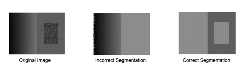
Although many methods had made considerable advances in segmenting images, most were slow and did not take into account that an object might have invariance in intensity and therefore would incorrectly segment that area.

To overcome the problems faced by previous methods, Felzenszwalb and Huttenlocher took a graph-based approach to segmentation. They formulated the problem as below:-

Let G = (V, E) be an undirected graph with vertices vi ∈ V, the set of elements to be segmented, and edges
(vi, vj ) ∈ E corresponding to pairs of neighboring vertices. Each edge (vi, vj ) ∈ E has a corresponding weight w((vi, vj )), which is a non-negative measure of the dissimilarity between neighboring elements vi and vj
.

In the case of image segmentation, the elements in V are pixels and the weight of an edge is some measure of the dissimilarity between the two pixels connected by that edge (e.g., the difference in intensity, color, motion, location, or some other local attribute).

S is a segmentation of a graph G such that G’ = (V, E’), where E’ ⊂ E . S divides G into G’ such that it contains distinct components (or regions) C. 

 

Graph Construction

Two approaches for constructing a graph out of an image were considered:

• Grid Graph: Each pixel is only connected with surrounding neighbors (8 other cells in total). The edge weight is the absolute difference between the intensity values of the pixels.

• Nearest Neighbor Graph: Each pixel is a point in the feature space (x, y, r, g, b), in which (x, y) is the pixel location and (r, g, b) is the color values in RGB. The weight is the Euclidean distance between two pixels’ feature vectors.

Some important concepts:-

Before learning about the criteria for a good graph partition, it is better to understand some concepts:

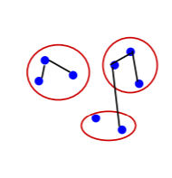
• Internal difference: Int(C) = max_e∈MST(C,E)w(e) , where MST is the minimum spanning tree of the components. A component ‘C’ can still remain connected even when we have removed all the edges with weights < Int(C). In other words, Internal Difference is the maximum edge weight that connects two nodes of the same component.

• Difference between two components: Dif (C1,C2)=min_{vi∈C1,vj∈C2,(vi,vj)∈E}w(vi,vj)  and   Dif(C1,C2)=∞ if there is no edge in-between. this can also be understood as the difference between two components. The difference between the two components is the minimum weight
  the edge that connects a node v_i
  in component C₁ to node v_j
  in C₂.

• Minimum internal difference:  MInt(C1,C2) = min(Int(C1) + τ(C1) , Int(C2) + τ(C2)) where τ(C)=k/|C|. This is the internal difference in the components C₁ and C₂. It is governed by a factork that we will understand a bit later.

Predicate for segmentation

To judge the quality of segmentation, a good pairwise region comparison is needed for two given regions say, C₁ and C₂:

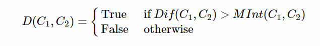
Only when this predicate is True, do we consider two components as independent. Otherwise, the segmentation is probably too fine and the components should be merged.

We have already defined the individual terms mentioned in the condition above, let’s now understand them better.

Difference between two components

The difference between the two components is the minimum weight edge that connects a node v_i in component C₁ to node v_j in C₂. 

 

Minimum Internal Difference

This is the internal difference in the components C₁ and C₂ governed by the factor k. This factor k in the definition of MInt separates the understanding Internal Difference and Minimum Internal Difference. As we saw earlier τ(C), sets the threshold by which the components need to be different from
the internal nodes in a component. We know that:

τ(C)=k/|C|,

here, the properties of this constant k are as follows:

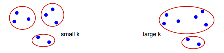
• If k is large, it causes a preference for larger objects.
•  k does not set a minimum size for components.

 

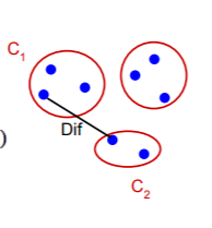
Now considering this, we can understand Minimum Internal Difference(MInt(C1,C2)) and Difference between two components(Dif(C1,C2))  in the same context:

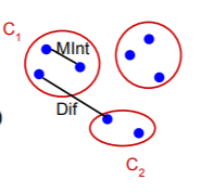
The above picture should make the predicate more clear to understand and visualize.

Only when the Difference between two components is greater that the Minimum Internal Difference of the two components, can the two components be divided into two different components.

Segmentation Algorithm and it’s working

We have already seen and understood the predicate, which is at the heart of this algorithm. Given an input graph G = (V, E), with n vertices and m edges. The output is a
segmentation of V into components S = (C1, . . . , Cr). The algorithm is as follows:

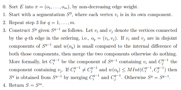
Although the algorithm can seem daunting at first, it is basically doing what the predicate wants:

The algorithm follows a bottom-up procedure. Given G=(V,E) and |V|=n, |E|=m. Where |V| is the number of vertices(pixels) and |E| is the number of edges.

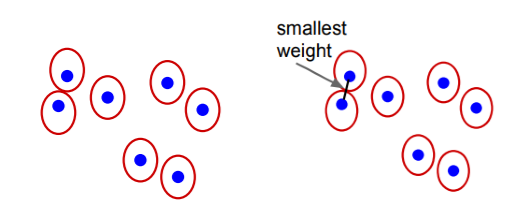
1. Edges are sorted by weight in ascending order, labeled as e₁,e₂,…,e_m.
2. Initially, each pixel stays in its own component, so we start with n components.
3. Repeat for k=1,…,m:

• The segmentation snapshot at step k is denoted as Sk.
• We take the k-th edge in the order, ek=(v_i , v_j).
• If v_i and v_j belong to the same component, do nothing and thus S^k=S^k−1.
• If v_i and v_j belong to two different components C_i^k−1 and C_j^k−1 as in the segmentation of S^k−1 we want to merge them into one if w(v_i,v_j) ≤ MInt(C_i^k−1,C_j^k−1); otherwise do nothing.

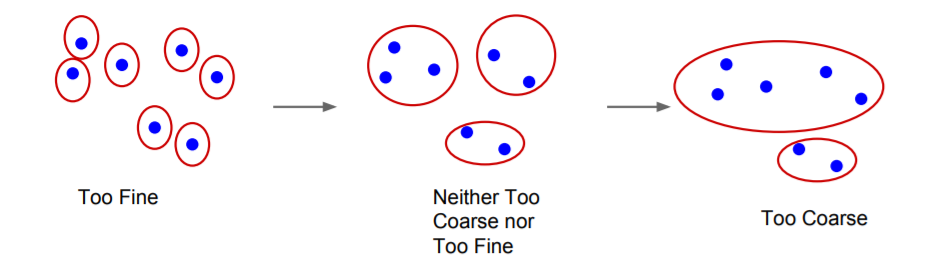
The entire segmentation process can be visualized as below:

 

This segmentation algorithm has many properties, the most important of them being:

For any (finite) graph G = (V, E) there exists some segmentation S that
is neither too coarse nor too fine.

For more properties and proofs, you can view the original paper.

This algorithm is very easy to implement, as it comes defined in skimage library.

#importing needed libraries
import skimage.segmentation
from matplotlib import pyplot as plt

#reading image
img = plt.imread("/content/image1.jpg")

#performing segmentation
#first for k=50
#seconf for k=1000
res1 = skimage.segmentation.felzenszwalb(img, scale=50)
res2 = skimage.segmentation.felzenszwalb(img, scale=1000)

#printing the results
fig = plt.figure(figsize=(12, 5))
ax1 = fig.add_subplot(121)
ax2 = fig.add_subplot(122)
ax1.imshow(res1); ax1.set_xlabel("k=50")
ax2.imshow(res2); ax2.set_xlabel("k=1000")
fig.suptitle("Graph based image segmentation")
plt.tight_layout()

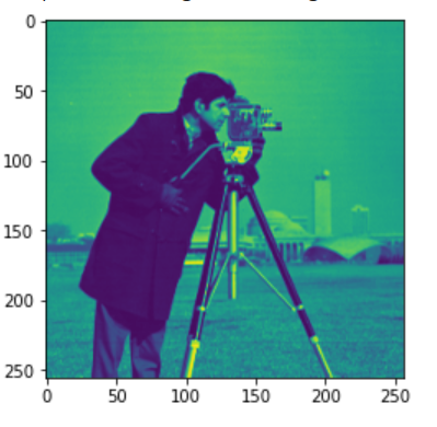
Original Image

 

Result

 

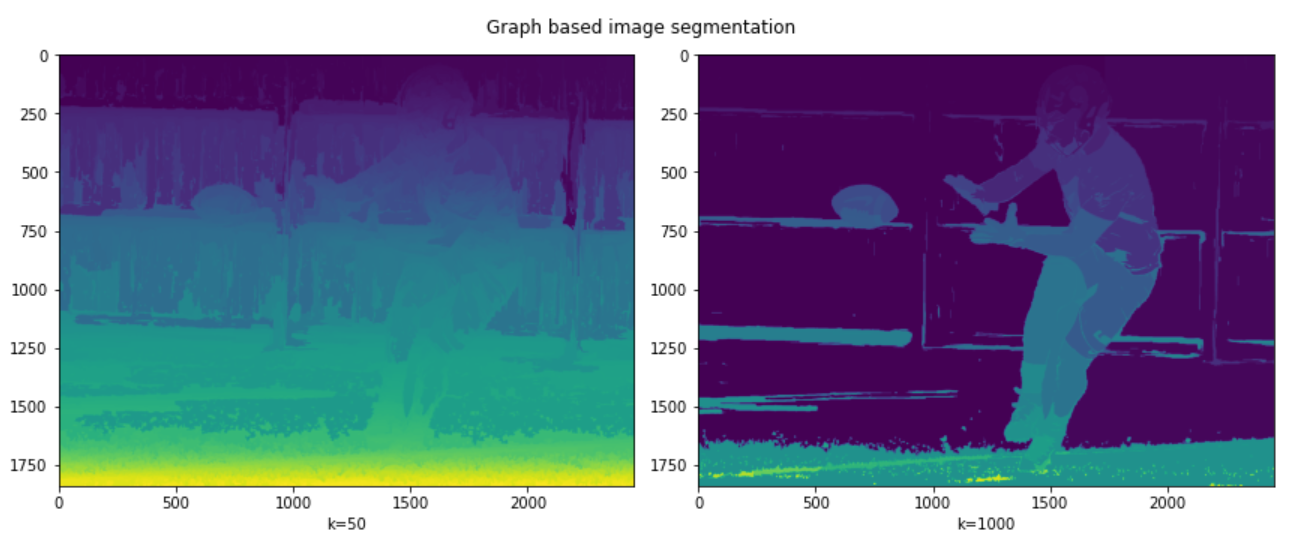
It can be seen in the results that a low value of k leads to coarser segmentation, while the large value of k leads to the selection of larger objects and is therefore finer. This can be seen from the ball being properly segmented in the second picture but not in the first.

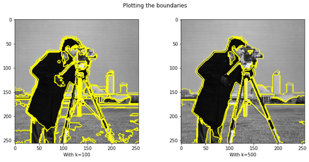
We can also mark the boundaries if we want:

from skimage.data import camera
from skimage.util import img_as_float
#import function for marking boundaries
from skimage.segmentation import mark_boundaries
img = img_as_float(camera()[::2, ::2])
res3 = skimage.segmentation.felzenszwalb(img, scale=100)
res4 = skimage.segmentation.felzenszwalb(img, scale=500)
fig = plt.figure(figsize=(12, 5))
ax1 = fig.add_subplot(121)
ax2 = fig.add_subplot(122)
ax1.imshow(mark_boundaries(img, res3)); ax1.set_xlabel("With k=100")
ax2.imshow(mark_boundaries(img, res4)); ax2.set_xlabel("With k=500")
fig.suptitle("Plotting the boundaries")

Original Image

 

Result

 

References

https://lilianweng.github.io/lil-log/2017/10/29/object-recognition-for-dummies-part-1.html#selective-search

https://davidstutz.de/implementation-of-felzenswalb-and-huttenlochers-graph-based-image-segmentation/ (for thumbnail)

About me

I am a sophomore at Birla Institute Of Technology, Mesra, currently pursuing Electrical and Electronics Engineering. My interests lie in the fields of Machine Learning and Deep Learning and like robotics.

You can connect with me at:

Linkedin

Github

Kaggle

You can also view some of the fun projects I worked on with my brother at:

https://www.youtube.com/channel/UC6J46NEyQEjag9fnOuBJ5hw

The media shown in this article on K-Means Clustering Algorithm are not owned by Analytics Vidhya and are used at the Author’s discretion.

SHIVAM SHANDILYA 27 May 2021