This article was published as a part of the Data Science Blogathon
Problem Statement
Everyone’s life revolves around their health. Good health is essential to all aspects of our lives. Health refers to a person’s ability to cope up with the environment on a physical, emotional, mental, and social level. Because of the quick speed of our lives, we are adopting many habits that are harming our health. One spends a lot of money to be healthy by participating in physical activities or having frequent health check-ups to avoid being unfit and get rid of health disorders. When we become ill we tend to spend a lot of money, resulting in a lot of medical expenses.
So, an application can be made which can make people understand the factors which are making them unfit, and creating a lot of medical expenses, and it could identify and estimate medical expense if someone has such factors.
Objective
· Predict the future medical expenses of subjects based on certain features building a robust machine learning model.
· Identifying the factors affecting the medical expenses of the subjects based on the model output.
Dataset-
For this project, the data has been imported from the machine learning repository. The dataset contains 1338 rows and 7 columns. The columns present in the dataset are ‘age’,’ sex’,’bmi’, ’children’, smoker’, ’region’, and ‘expenses’. The Expenses column is the target column and the rest others are independent columns. Independent columns are those which will predict the outcome.
The first column is Age. Age is an important factor for predicting medical expenses because young people are generally more healthy than old ones and the medical expenses for Young People will be quite less as compared to old people.
The Next column is sex, which has two Categories in this column: Male and Female. The sex of the person can also play a vital role in predicting the medical expenses of a subject.
After that, you have the ‘bmi’ column, then BMI is Body Mass Index.
For most adults, an ideal BMI is in the 18.5 to 24.9 range.
For children and young people aged 2 to 18, the BMI calculation takes into account age and gender as well as height and weight. If your BMI is less than 18.5, you are considered underweight. People with very low or very high ‘bmi’ are more likely to require medical assistance, resulting in higher costs.
The fourth column is the ‘children’ column, which contains information on how many children your patients have. Persons who have children are under more pressure because of their children’s education, and other needs than people who do not have children.
The fifth is the ‘smoker’ column. The Smoking factor is also considered to be one of the Most Important factors as the people who smoke are always at risk when their age reaches 50 to 60.
Next is the ‘region’ column. Some Regions are Hygienic, Clean, Neat, and Prosperous, But some Regions are not, and this information affects health which is related to medical expenses.
DatasetDownloadLink: https://drive.google.com/uc?id=1WJxHVqSZNkTRLWIdlJR0VIW0vcaCGRPz
Data Visualization
Ø Univariate Analysis:
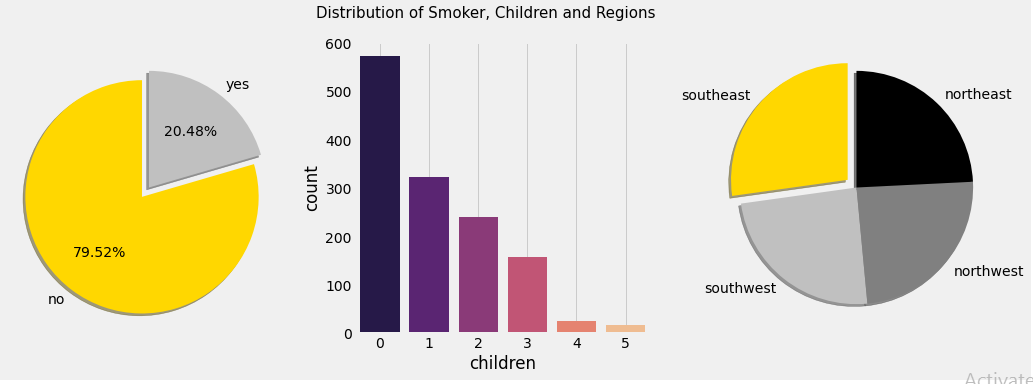
Here we have used a pie chart to plot the Smoker Column, as the Smoker column has only two values: Yes and No. We have found 20.48% of the subjects are smokers and 79.52 % are non-smoker.
Using a Count plot we have shown the subjects having children ranging from 0 to 5 and it has been computed and observed from the count plot also that those who are having no children are highest in number.
- Number of Subjects having no children- 574
- Number of Subjects having one child- 324
- Number of Subjects having two children- 240
- Number of Subjects having three children- 157
- Number of Subjects having four children- 25
- Number of Subjects having five children-18
- We have again used a pie chart to plot the number of inhabitants in the region column which consists of four segments: Northeast, Northwest, Southeast, Southwest
The number of Southwest and Northwest are the same and the value is 324, but the number of inhabitants in Northeast and Southeast are respectively 324 and 364.
The three plots are shown below.
Again the distribution of Age, BMI, and Expenses have been shown using the distribution plot. The following things are observed from those distribution plots:
§ We have an equal number of people of all ages.
§ The BMI of the patients seems to be normally distributed where maximum people have BMI around 30 and very few people have less BMI around 10, similarly very few people have high BMI around 60.
§ Expenses column seems to be right-skewed. Here log transformation has been applied to make this distribution normal so it doesn’t create any problem while predicting.
The Distribution plots are shown below:
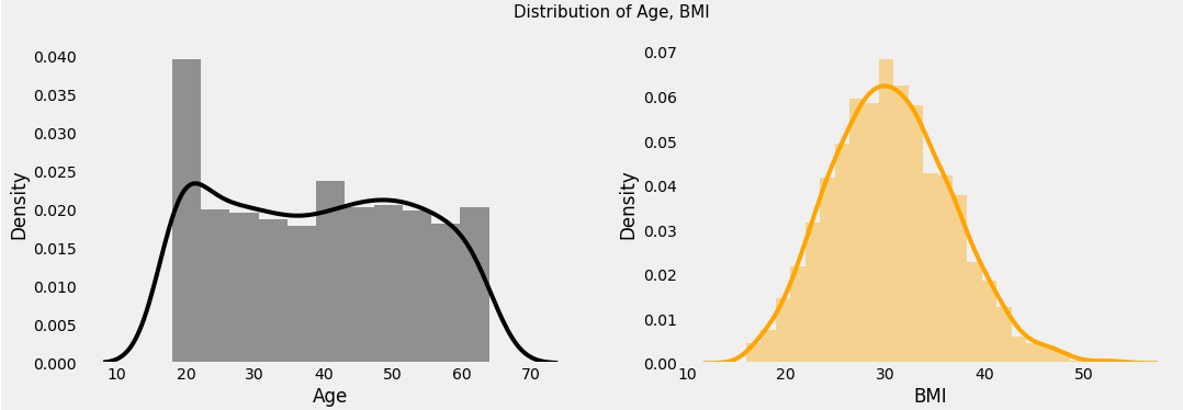
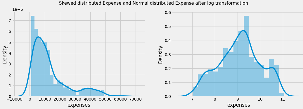
Fig 2(a) Distribution of Smoker, Children, and Regions, 2(b) Skewed
distributed Expense log Transformed Expense
Ø Bivariate Analysis:
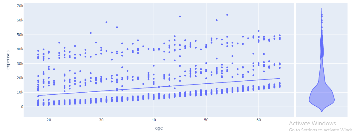
Scatter plots have been used to show the variation of expenses with age. Here we have used the Plotly library. It has been noticed that with an increase in age the medical expenses have increased but some people are of higher age but have lower medical expenses. The advantage of the Plotly chart is that we can add some parameters such as trend line and while hovering over the trend line it was observed that the expense and age have a linear relationship.
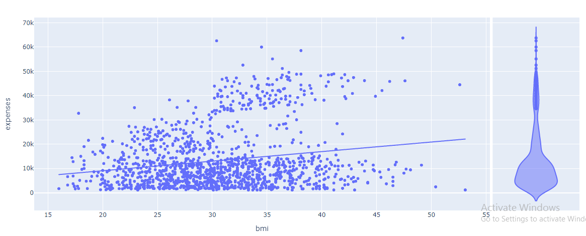
We have also plotted the scatterplot between BMI and expenses and it has been noticed that most of the data is situated at the bottom of the trend line indicating that people with high, low, and medium BMI can have low expenses, which is an irregular pattern, but if we take a look at the trend line we can notice that people with high BMI, their medical expense will be high, so we can conclude that for people with high BMI the expenses may be increased but in rare case.
We have also tried to understand the relationship between categorical and numerical variables through bivariate analysis.
The plots are shown below.
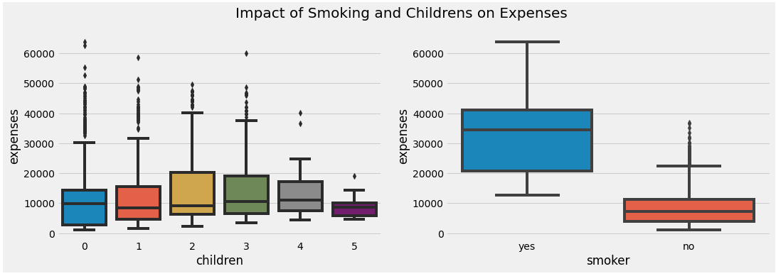
We plotted the bar plot between the children and expenses and it has been noticed people with more number of children the expense is more as with more children parents need to take care of the health of all of them rather those who have no children or one child, but as there is very less number of people who are having more than 3 children so for them the expense is almost same so we capped them. The people with 3 children have the highest expenses among them.
We have also seen the relationship between smokers and expenses through box plots and it has been noticed that for smokers the expense is much high than nonsmokers as it is obvious because smoking is injurious to health so smokers are likely to have health issues than nonsmokers causing their medical expenses to increase.
The plots are shown
below.
Ø Multivariate Analysis:
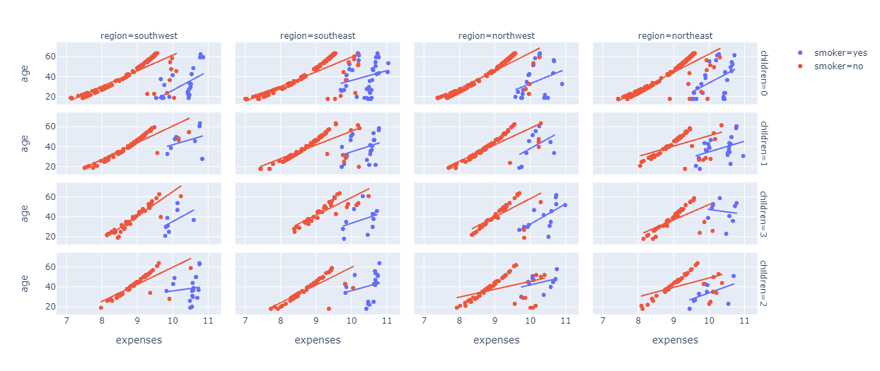
A scatter plot has been created between the age and expenses column, Specifying the smoker column to impart color in data points. If the patient is a smoker, he or she will be specified with Blue color, and if the patient is a non-smoker, then he or she will be specified with Red color. After that, add faceting layers. the “children” column has been added as a facet on the row side, whereas the “Region” column has been added as a facet on the column side.
If we look at the Charts Carefully, we can easily figure out that the Expenses of Smokers in most of the regions ranges from 10 thousand to 11 thousand. Whereas the Expenses of Non Smokers in most of the regions ranges from 9 thousand to 10 thousand and Finally, If you look at the trend lines, you can see that In general if the age is less, the Expense would also be less. Moreover, subjects who smoke and those who are a nonsmoker but belong to the same age medical expense is more for those who are smokers than the nonsmoker ones.
The plot is shown below:
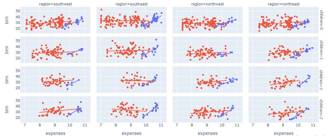
After that, again created a similar kind of scatter plot, where we plotted BMI in the place of age.
Looking at the chart, you can clearly see that there is an increasing pattern for BMI as well.
For smokers with less BMI, the expenses are around 9.5 thousand rupees.
For smokers with high BMI, the expenses are around 11 thousand rupees.
For nonsmokers, BMI is not a huge factor, their expenses range from 7k to 10k.
The plot is shown below:
We have used the Bubble chart to represent the relation of expense with BMI, age, and smoking.
It is noticed from the chart that BMI is not a powerful factor as people having less BMI also have high medical expenses and it is very clear from the chart that people who smoke definitely have high medical expenses. Moreover, the size of the bubble indicates age and it has been noticed that with an increase in bubble size that means with an increase in age medical expenses increase.
The plot is shown below:
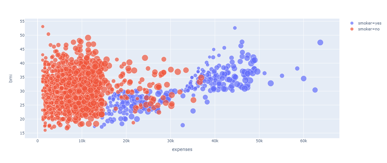
Fig 7. Relation of Expense with BMI, age, and smoking
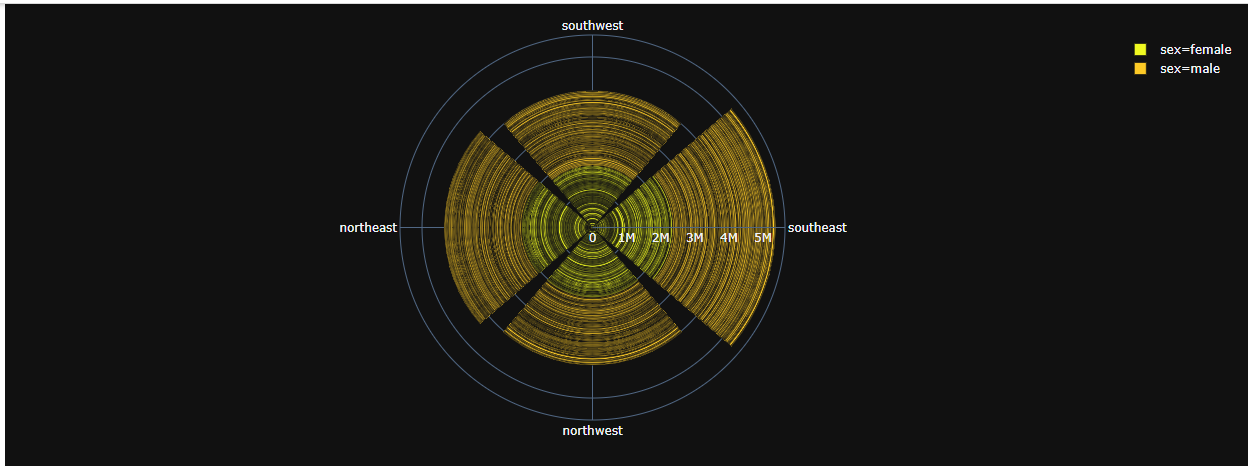
Again we have plotted a Bar Polar chart and from that, it can be easily understood that the southeast region has higher medical expenses compared to all the other regions, and also the males have higher expenses in general in almost all the regions.
The plot is shown below.
Use the group by function and group the data using the region column and use the aggregate function and specify the minimum, mean and maximum aggregation of expenses.
These Aggregations will help to understand whether you should perform Capping in the Region Column or not.
Now, we can notice that the maximum expenses are in the southeast region while other regions also have comparably high expenses.
So, there is no huge difference between the expenses in any region.
But, if we take a look at the Mean of the Expenses, the Expenses in the Southeast Region is very high, whereas, in all the other regions, It is very low.
Hence, concluding that the People in the Southeast region have very high expenses as compared to people living in other regions. So, we can cap all the Other three Regions that is the Southwest Region, the Northeast Region, and the Northwest Region, as the Expenses in these three regions are very similar to each other.
We have also computed the expenses for different sex categories using the group by function on sex column and notice male has more expense than female.
Similarly, we computed expenses for smokers and nonsmokers grouping by smoker column and found smokers have more medical expenses than nonsmokers.
Also, we calculated expenses for those subjects having children grouping by children column and found with more children expense tend to increase. The skewness and
kurtosis also has been checked for each of the columns.
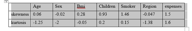
Most of the subjects were aged between 20 to 60 and the distribution are normal and the distribution curve was flatter causes negative kurtosis.
Most of the subjects having BMI between 20 to 40 and the distribution is almost normal and the curve was not flat.
Most of the expenses were right-skewed which means for more no of the subject’s expenses lie between 5000 to 20000 and for a few of them it was 40000 and the curve was peaked.
Data Pre-processing
Ø Encoding of categorical columns
In our dataset, we have three categorical columns: Sex, Smoker, and Region
Sex consists of males and females and it has been observed from the data analysis that males have higher medical expenses than females. As a result, we have encoded male as 2 and female as 1.
The Smoker column consists of smokers and nonsmokers and it has been observed the smoker has more medical expenses than the nonsmoker ones so we encoded smokers as 2 and nonsmokers as 1.
The Region column comprises four segments: Southeast, Southwest, Northeast, Northwest.
It has been noticed from the data analysis the Southeast region has the highest expenses followed by Northeast, Northwest, and Southwest, so we have encoded those regions as 4,3,2,1 respectively.
Ø Data Splitting
We have split the data in the entire dataset in Train and Test with a ratio of 80:20. We have trained the model with trained data and then we applied the model to the test dataset to check the performance of the model.
Ø Feature Scaling
Feature scaling is a method used to normalize the range of independent variables or features of data. Feature Scaling basically helps to normalize the data within the same scale. We have used the fit_transform function to apply feature scaling on the training data but used the transform function to apply feature scaling on the testing data because the fit_transform function will first learn all the patterns in the data and then it will apply feature scaling on the data. But, we cannot use the fit_transform function for testing data as you cannot learn the patterns from these data.
Hypothesis Testing
Ø t-Test
The t-Test has been done on the sex and smoker column with the target column expense to find if there is any association of these two columns with the target column.
The sex column comprises two variables male and female. We assumed the Null Hypothesis that the mean expense for both males and females is the same. After applying t-Test we found p-value 0.036 which is less than 0.05 which rejects NULL Hypothesis, that means the mean expense of male and female is different.
The smoker column comprises two variables yes and no which means smoker and nonsmoker. We assumed the Null Hypothesis that the expense for both smoker and nonsmoker is the same After applying the t-Test it has also been found that the p-value yielded as 8.27e-283 which is much less than 0.05 which rejects NULL Hypothesis that means the mean expense for who smokes and those who don’t smoke is different.
Ø ANOVA
When there are more than two variables we apply the ANOVA test. Here on the region and children column, ANOVA test was done with the target column expense.
In the children column, we have four variables 0,1,2,3 which means subjects having no children to 3 children, and the assumption of NULL Hypothesis was the expense for those having no children, one child, two children, three children is same. After applying the F test it was found F statistic value was 4.54 and the p-value of F statistic was 0.0035 which is much less than the 0.05 so we reject NULL Hypothesis which means that the expense for those having no children, one child, two children, three children is not same.
In the same way, we applied the F test on the region column which we encoded as 4,3,2,1 for southeast, northeast, northwest, southwest respectively. We assumed Null Hypothesis that the expense of all four regions is the same, but after applying the F test we found the F statistic value as 2.96 and the p-value of F statistic as 0.03 which is less than 0.05 so the NULL Hypothesis got rejected and we concluded that the expenses of these four regions are different.
Ø Chi-Square Test
Chi-square test is done among categorical variables two find any kind of association among them. Here Sex and Smoker columns were chosen for applying this test and the assumption for NULL Hypothesis was there is no relationship between Sex and Smoker column but the chi-square statistic value was found as 7.76 which was more than the critical value of 3.84 and also the p-value was obtained as 0.005 which is less than 0.05. This validates that the NULL hypothesis is rejected which means there is some association between these two categorical variables.
Model Building
Ø Linear Regression:
Linear Regression was applied to predicted Future Medical Expenses for your Patients based on certain features such as Age, Gender, Region, Smoking Behavior, and Number of children.
We computed R2 and RMSE values which were obtained as 0.79 and 5673.09 which means 79 % of the variation of target column expense can be well explained by one of the predictor variables. And RMSE interprets that the expected expense can be more or less than 5673 of the actual expense.
We then use the stats model to find a summary of the linear regression model and the following are found.
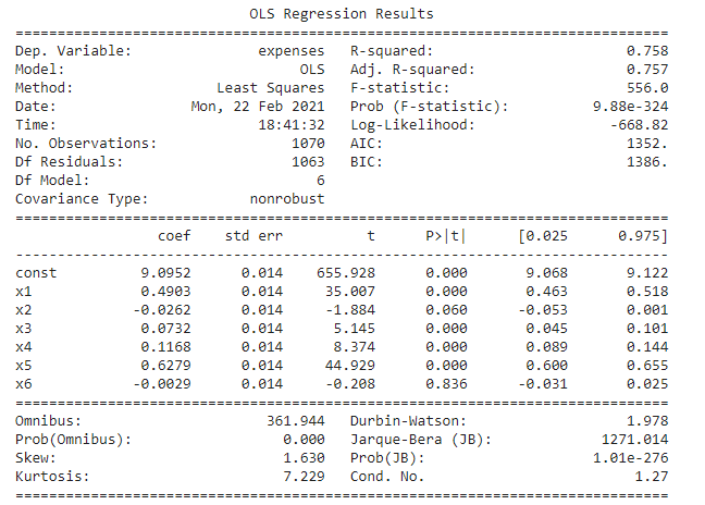
Fig 9(a). Regression_summary_1
Here we found for two variables sex and region we got a p-value of more than 0.05 which means these are insignificant, so to confirm this we did a variance inflation factor test on the independent variables to show the multicollinearity and the result is below.
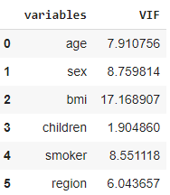
and it was found that the BMI column showed a value of 17 which is more than 10 so we dropped that from the dataset and again did linear regression and found summary and noticed the following result.
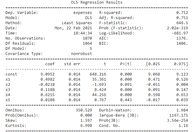
From the above summary, we get to see sex and region column are showing insignificant as p values are >0.05 so these two columns have been dropped and the linear regression was done again. Following is the result.
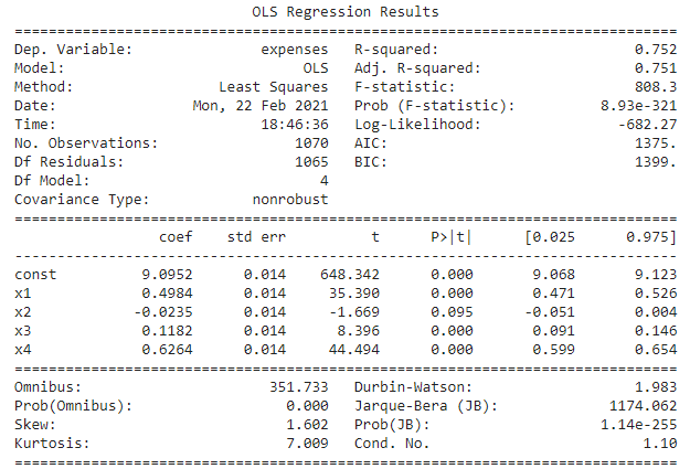
From the above result, it is again observed that the ‘sex’ column remains insignificant so it was dropped and the regression was run again. Following is the result of that regression.
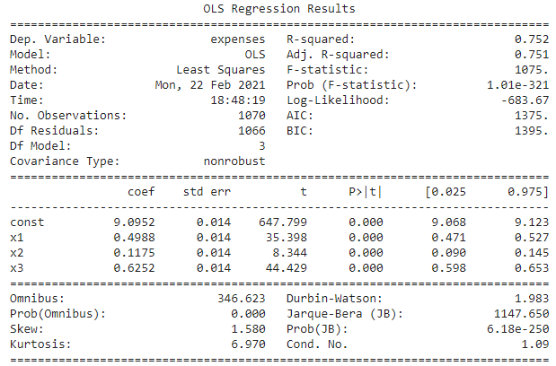
1.p-value for F statistic is < 0.05 (we will consider 0.5 as significance level for this project) so we can say that our model is significant (at least for one independent variable the regression coefficient. is not equal to zero, rejecting the null hypothesis, The null hypothesis under this is “all the regression coefficients are equal to zero”.) In our case, The F statistic value is 1075, and Prob(F-Statistics) is much less than 0.05 so we can say our model is quite significant.
2. R-squared value is 0.778 which means 77.8 % variation of output can well be explained by independent variables of the model.
3. If the Adjusted R2 is much less than the R square value it means there are variables in the dataset which is irrelevant to the model, which are not impacting the target variable. In our case, the R square value is 0.752 and the adjusted R-square is 0.751 which means our model has no irrelevant features which are not explaining the target output.
4.Now we will check p values for each attributes if the p values are <0.05 we will say that the attribute is contributing to the model (reject the null hypothesis(coef=0)) if > 0.05 then the attribute is insignificant (accept the null hypothesis(coef=0)).In our model there is no feature which is having p-value > 0.05 which means there is a linear relationship of target variable with all the features.
5.Prob(Omnibus): One of the assumptions of OLS is that the errors are normally distributed. an Omnibus test is performed to check this. Here, the null hypothesis is that the errors are normally distributed. Prob(Omnibus) is supposed to be close to the 1 for it to satisfy the OLS assumption and in our case, its 0 and Omnibus value is also high which is supposed to be close to 1 indicates that our data is heteroskedastic.
6.Durbin-Watson: Another assumption of OLS is No Autocorrelation in the residuals. A value of 2 is preferred and in our case, it’s 1.983 so there is no autocorrelation in errors, we verified it also with the Durbin-Watson Test written later.
7.Prob(Jarque-Bera): It is like the Omnibus test. It is used to confirm the Omnibus test result. It is used to check if the errors are is normally distributed. A large JB value indicates that errors are not normally distributed. In our case, we obtain a JB value of 1147.65 which indicates that our data errors are heteroscedastic.
8.Condition Number: This test measures the sensitivity of a function’s output as compared to its input (characteristic #4). When we have multicollinearity, we can expect much higher fluctuations to small changes in the data, hence, we hope to see a relatively small number, something below 30 and in our case, it’s 1.16 so there is no multicollinearity in our dataset.
9. Log-Likelihood: More negative the log-likelihood better the model. In our case, its value is -683.17 which makes the model better.
10. AIC & BIC score- Less the AIC/BIC score better the model will be. The lowest between the two is to choose. In our case, it’s low which increases the model performance.
The linear equation that we finally found as below,
expenses= 9.09+49*age+0.12*children+0.62*smoker
Homoscedasticity Test:
A residual plot has been drawn to check heteroscedasticity which means there are variances among errors that shouldn’t be there. The plot shows the presence of heteroscedasticity in the data and shown below.
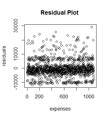
Fig 10. Residual Plot
To confirm the presence of Heteroscedasticity we applied a test named Breusch pagan test. The NULL Hypothesis for this is error variances are equal. But we found BP=211.94 and p-value as <2.2e-16 which is less than 0.05 which rejects the null hypothesis so it also confirms that data is heteroscedastic.
Autocorrelation Testing:
One of the assumptions of linear regression is that there should be no autocorrelation among errors of the data, and there is a test called Durbin-Watson Test to check this. The Null hypothesis for this test is there is no autocorrelation among residuals and after applying this test we found DW=2.1069 and p-value as 0.9603 which is more than 0.05 so the NULL hypothesis got accepted which means there is no autocorrelation among residuals.
Normality Testing:
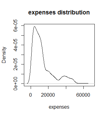
Fig 11(a). Distribution of Expense
It has been found from the above plot that the target column is right-skewed, not normally distributed, but we applied the Shapiro Wilk test to confirm that. The NULL Hypothesis for that test states that the data are normally distributed. But we found w=0.81469 and p-value <2.2e-16 which is less than 0.05 which means NULL Hypothesis got no support so data are not normally distributed.
We log-transformed the target column ‘expenses’ to make it normal and checked with the Shapiro Wilk test again but the result again showed the column is not normally distributed.
The log-transformed pic is given below.
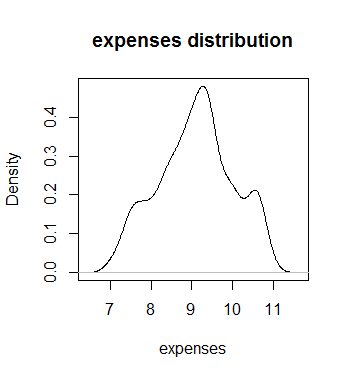
We can use BoxCox Transformation to make the data normal and we found the lambda value =0 which should lie between -2 to 2 but after that also we couldn’t make the data normal. Breusch Pagan test again failed.
The RMSE value found as 5784.876
So our linear regression model will not give a good result as there is heteroscedasticity and data is not normal so We applied a few more models to get a better prediction.
Random Forest Regressor
Random Forest is an ensemble learning method for classification and regression by constructing multiple numbers of decision trees at training time and
Outputting the average prediction of the individual trees in case of regression whereas outputting the class that is the mode of the classes in case of classification.
It is one of the Most powerful Machine Learning algorithms which works well in most cases.
First of all, the RandomForestRegressor package was imported from sklearn. ensemble library, so that we can use this model to predict the Expenses.
After that, we specified a Model using this Random Forest Regressor Class.
Now, as the Model is Ready, trained our Model using the Training data, for that fit function, was used and used the training data.
Here, the Training Data refers to x_train and y_train.
Where x_train is the independent variable, and Y_train is the dependent variable or target variable.
After the Model gets trained, we started performing Predictions using this Predictive Model created using the Random Forest Regressor.
To do that, used predict function and specified the independent variables inside the function, to get the predictions and saved the result produced by the Random forest in a new variable, so that we can compare the Results later if required.
After building the predictive model, evaluated the Model using various Performance Metrics.
In this case, we checked the R2 score and RMSE Score as in the case of the linear regressor.
In the case of the Random Forest model, the RMSE score comes out to be 0.4188 whereas the r2 score comes out to be 0.79 which makes it clear that Random Forest works much better than Linear Regression for this Dataset.
Gradient Boosting Regressor
- Gradient
Boosting is a very popular Boosting technique. - It
works by sequentially adding the previous predictors under fitted
predictions to the ensemble ensuring that the errors made previously are
corrected.
Random Forest is also an Ensemble, But In Random Forest the Ensembling happens Parallelly,
But, In the case of Gradient Boosting, the Ensembling happens Sequentially, which means that the First Model’s Errors will be used to Build the Second Model and the Second Model’s Error will be used to Build the Third Model, and so on. The Models will be built until and unless the Errors are optimized in the best way.
That means By using the Gradient Boosting Models we can make the least error possible.
First of all, Using the Gradient Boosting Regressor Model is to be imported from the sklearn.ensemble library.
After that, make a Base Gradient Boosting Regressor Model, and then we trained this Model using the fit function on the Training Data that is x_train and y_train.
Where, X_train is your Independent Variable, and y_train is your Dependent Variable.
After the Model is built we predicted the Target Variable for our test data using the predict function and save the result in a new variable, so that to compare the results later.
After that, we performed Model Evaluation using the R2 score and RMSE score Performance Metrics as did for the Last Two Models and we obtained the RMSE Score as 0.3744, whereas the R2 score comes out to be 0.832.
Cross-validation: –
Cross-validation is a resampling procedure that is used to evaluate our machine learning models on limited data samples.
The goal of cross-validation is to test the model’s ability to predict new data that was not used in estimating it.
It has a single parameter called ‘k’, which indicates the number of groups that the data would be split into, here we train the model on k-1 datasets and test on the kth dataset and this process repeats till the k value we set and in our case, we selected k value as 5
To perform cross-validation, import the cross_val_score from sklearn.model_selection and run a for loop through each of the three models output using cv =5 to choose the best model and computed mean cv scores for each of the models after the loop iterates for 5 times and we found Gradient Boosting Regressor was showing best cv score as 0.79 which proves Gradient Boosting Regressor is the best model in predicting medical expenses among three.
Comparing Performance of three models:
We have created a NumPy array of the r2 score of all three models, Linear Regression, Random Forest, and Gradient Boosting.
An array for the labels was also created as well, to compare these Values using bar charts.
After that, using the argsort function, values have been sorted and specified in the color palette.
Here a Rainbow palette has been used and the Bar plot built using the seaborn Library shows a higher r2 score value for Gradient Boosting and lowest for Linear Regression.
That means, the Gradient Boosting Model, is the Best Choice whereas the Linear Regression Model is the worst for this Case thus we have successfully built our predictive model and compared these predictive models based on their accuracies and Results. Below is the bar plot to show the performance of the three used models.
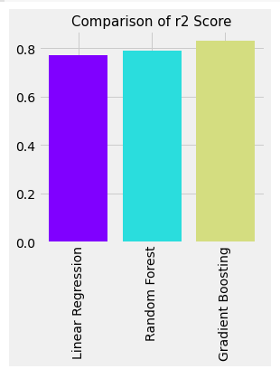
Fig 12. Comparison of R2 Score of three models
Model Deployment:
An app has been developed using Flask and it was designed to develop an HTML page, both were done on Pycharm Editor for user convenience that allows users to predict the possible medical costs by plugging in basic details such as age, sex, region, smoking status (smoker or non-smoker), BMI, and a number of children and then pressing a submit button out there. The App has been implemented through the Amazon-AWS platform so users from anywhere any get their probable medical health expense accessing the link of the app.
Conclusion:
We came to know that the Most Important Factor to Predict the Medical Expenses of a subject is Smoking Behavior and Age, that means, smoking is Bad for Health, as already know that and which inevitably increases medical expenses as due to smoking one is likely to fall ill more than the nonsmokers.
We also found that with increasing of age, one needs to take some more care and precautions for your health as with the increase of age health becomes fragile so they go for frequent medical check-up, likely to fall ill quickly as with the increase of age immunity falls so they adopt measures to stay healthy by taking medicines and engaging in some physical activities like jogging, walking, Yoga which causes an increase of medical expenses.
Apart from that you also understood that Gender, Number of Children, the Region also have a good impact on determining Medical Expenses.
We have built three models among which the Gradient Boosting Regressor model shows the best result through which we can say 83.2% variability of expenses can well be explained by predictor variables and which yields comparatively low RMSE value so our predicted expense through this model will not vary too much from the actual expense.
My LinkedIn Profile ID: https://www.linkedin.com/in/ananda-chatterjee-b5813355/
The media shown in this article are not owned by Analytics Vidhya and are used at the Author’s discretion.


