This article was published as a part of the Data Science Blogathon.
What are GANs?

Figure 1: Images generated by a GAN created by NVIDIA.
In machine learning, GAN modeling is an unsupervised learning task that contains learning the regularities or discovering the patterns in input data automatically in such a way that the model can generate or output new examples that are drawn from the original dataset.
GANs are an interesting and rapidly gaining attention, bringing on the promise of these generative models in their skill to generate synthetic as well as real examples across a range of problems in different domains, very good example of GANs are in image-to-image translation tasks such as generating photorealistic photos of objects, scenes, translating photos of summer to winter or day to night, and people that even humans cannot differentiate that they are fake.
Types of GAN:
– Generative Adversarial Network (GAN)
– Deep Convolutional Generative Adversarial Network (DCGAN)
– Conditional Generative Adversarial Network (cGAN)
– Information Maximizing Generative Adversarial Network (InfoGAN)
– Auxiliary Classifier Generative Adversarial Network (AC-GAN)
– Stacked Generative Adversarial Network (StackGAN)
– Context Encoders
– Pix2Pix
– Wasserstein Generative Adversarial Network (WGAN)
– Cycle-Consistent Generative Adversarial Network (CycleGAN)
– Progressive Growing Generative Adversarial Network (Progressive GAN)
– Style-Based Generative Adversarial Network (StyleGAN)
– Big Generative Adversarial Network (BigGAN)
Here we will implement Progressive GAN from the scratch.
What is ProGAN?
Progressive Growing GAN also know as ProGAN introduced by Tero Karras, Timo Aila, Samuli Laine, Jaakko Lehtinen from NVIDIA and it is an extension of the training process of GAN that allows the generator models to train with stability which can produce large-high-quality images.
It involves training by starting with a very small image and then the blocks of layers added incrementally so that the output size of the generator model increases and increases the input size of the discriminator model until the desired image size is obtained. This type of approach has proven very effective at generating high-quality synthetic images that are highly realistic.
It basically involves 4 major steps
1) Progressive growing (of model and layers)
2) Minibatch std on Discriminator
3) Normalization with PixelNorm
4) Equalized Learning Rate
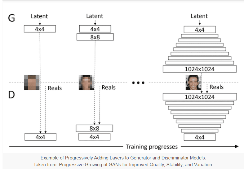
Here we can see in the above figure that Progressive Growing GAN involves using a generator and discriminator model with the traditional GAN structure and its starts with very small images, such as 4×4 pixels.
During the training process, it systematically adds new blocks of convolutional layers to both the generator model and the discriminator model. This incremental addition of the convolutional layers allows the models to learn coarse-level detail effectively at the beginning and later learn even finer detail, both on the generator and discriminator side.

The process of adding a new block of layers involves the usage of skip connection as shown in the above figure, it is mainly to connect the new block either to the output of the generator or the input of the discriminator and adding it to the existing output or input layer with a weighting which controls the influence of the new block.
This technique is demonstrated in the figure above, taken from the paper.
It shows a generator that outputs a 16×16 image and a discriminator that takes a 16×16 pixel image. The models are grown to the size of 32×32.
Let’s start the implementation
We will be implementing using Pytorch, First, we need to create separate classes for each of the following:
– 2d Convolutional layer
– Pixel Norm
– Generator
– Discriminator
Create a python file with the name ‘progessive_GAN’, Below code has four classes which are mentioned above and this is used for training the ProGan network.
import torch
import torch.nn as nn
import torch.nn.functional as F
from math import log2
factors = [1, 1, 1, 1, 1/2, 1/4, 1/8, 1/16, 1/32]


class WSConv2d(nn.Module):
def __init__(self, input_channel, out_channel, kernel_size=3 , stride=1, padding=1, gain=2):
super(WSConv2d, self).__init__()
self.conv = nn.Conv2d(input_channel, out_channel, kernel_size, stride, padding)
self.scale = (gain / (input_channel * (kernel_size ** 2))) ** 0.5
self.bias = self.conv.bias
self.conv.bias = None

# conv layer
nn.init.normal_(self.conv.weight)
nn.init.zeros_(self.bias)

def forward(self, x):
return self.conv(x * self.scale) + self.bias.view(1, self.bias.shape[0], 1, 1)


class PixelNorm(nn.Module):
def __init__(self):
super(PixelNorm, self).__init__()
self.epsilon = 1e-8

def forward(self, x):
return x / torch.sqrt(torch.mean(x ** 2, dim=1, keepdim=True) + self.epsilon)


class CNNBlock(nn.Module):
def __init__(self, input_channel, out_channel, pixel_norm=True):
super(CNNBlock, self).__init__()
self.conv1 = WSConv2d(input_channel, out_channel)
self.conv2 = WSConv2d(out_channel, out_channel)
self.leaky = nn.LeakyReLU(0.2)
self.pn = PixelNorm()
self.use_pn = pixel_norm

def forward(self, x):
x = self.leaky(self.conv1(x))
x = self.pn(x) if self.use_pn else x
x = self.leaky(self.conv2(x))
x = self.pn(x) if self.use_pn else x
return x


class Generator(nn.Module):
def __init__(self, z_dim, in_channels, img_channels=3):
super(Generator, self).__init__()

# initial takes 1x1 -> 4x4
self.initial = nn.Sequential(
PixelNorm(),
nn.ConvTranspose2d(z_dim, in_channels, 4, 1, 0),
nn.LeakyReLU(0.2),
WSConv2d(in_channels, in_channels, kernel_size=3, stride=1, padding=1),
nn.LeakyReLU(0.2),
PixelNorm(),
)

self.initial_rgb = WSConv2d(
in_channels, img_channels, kernel_size=1, stride=1, padding=0
)
self.prog_blocks, self.rgb_layers = (
nn.ModuleList([]),
nn.ModuleList([self.initial_rgb]),
)

for i in range(
len(factors) - 1
): # -1 to prevent index error because of factors[i+1]
conv_in_c = int(in_channels * factors[i])
conv_out_c = int(in_channels * factors[i + 1])
self.prog_blocks.append(CNNBlock(conv_in_c, conv_out_c))
self.rgb_layers.append(
WSConv2d(conv_out_c, img_channels, kernel_size=1, stride=1, padding=0)
)

def fade_in(self, alpha, upscaled, generated):
# alpha should be scalar within [0, 1], and upscale.shape == generated.shape
return torch.tanh(alpha * generated + (1 - alpha) * upscaled)

def forward(self, x, alpha, steps):
out = self.initial(x)

if steps == 0:
return self.initial_rgb(out)

for step in range(steps):
upscaled = F.interpolate(out, scale_factor=2, mode="nearest")
out = self.prog_blocks[step](upscaled)

final_upscaled = self.rgb_layers[steps - 1](upscaled)
final_out = self.rgb_layers[steps](out)
return self.fade_in(alpha, final_upscaled, final_out)


class Discriminator(nn.Module):
def __init__(self, z_dim, in_channels, img_channels=3):
super(Discriminator, self).__init__()
self.prog_blocks, self.rgb_layers = nn.ModuleList([]), nn.ModuleList([])
self.leaky = nn.LeakyReLU(0.2)

# here we work back ways from factors because the discriminator
# should be mirrored from the generator. So the first prog_block and
# rgb layer we append will work for input size 1024x1024, then 512->256-> etc
for i in range(len(factors) - 1, 0, -1):
conv_in = int(in_channels * factors[i])
conv_out = int(in_channels * factors[i - 1])
self.prog_blocks.append(CNNBlock(conv_in, conv_out, pixel_norm=False))
self.rgb_layers.append(
WSConv2d(img_channels, conv_in, kernel_size=1, stride=1, padding=0)
)

# perhaps confusing name "initial_rgb" this is just the RGB layer for 4x4 input size
# did this to "mirror" the generator initial_rgb
self.initial_rgb = WSConv2d(
img_channels, in_channels, kernel_size=1, stride=1, padding=0
)
self.rgb_layers.append(self.initial_rgb)
self.avg_pool = nn.AvgPool2d(
kernel_size=2, stride=2
) # down sampling using avg pool

# this is the block for 4x4 input size
self.final_block = nn.Sequential(
# +1 to in_channels because we concatenate from MiniBatch std
WSConv2d(in_channels + 1, in_channels, kernel_size=3, padding=1),
nn.LeakyReLU(0.2),
WSConv2d(in_channels, in_channels, kernel_size=4, padding=0, stride=1),
nn.LeakyReLU(0.2),
WSConv2d(
in_channels, 1, kernel_size=1, padding=0, stride=1
), # we use this instead of linear layer
)

def fade_in(self, alpha, downscaled, out):
return alpha * out + (1 - alpha) * downscaled

def minibatch_std(self, x):
batch_statistics = (
torch.std(x, dim=0).mean().repeat(x.shape[0], 1, x.shape[2], x.shape[3]))
return torch.cat([x, batch_statistics], dim=1)

def forward(self, x, alpha, steps):
cur_step = len(self.prog_blocks) - steps

out = self.leaky(self.rgb_layers[cur_step](x))

if steps == 0: # i.e, image is 4x4
out = self.minibatch_std(out)
return self.final_block(out).view(out.shape[0], -1)

downscaled = self.leaky(self.rgb_layers[cur_step + 1](self.avg_pool(x)))
out = self.avg_pool(self.prog_blocks[cur_step](out))
out = self.fade_in(alpha, downscaled, out)

for step in range(cur_step + 1, len(self.prog_blocks)):
out = self.prog_blocks[step](out)
out = self.avg_pool(out)

out = self.minibatch_std(out)
return self.final_block(out).view(out.shape[0], -1)


if __name__ == "__main__":
Z_DIM = 100
IN_CHANNELS = 256
gen = Generator(Z_DIM, IN_CHANNELS, img_channels=3)
critic = Discriminator(Z_DIM, IN_CHANNELS, img_channels=3)

for img_size in [4, 8, 16, 32, 64, 128, 256, 512, 1024]:
num_steps = int(log2(img_size / 4))
x = torch.randn((1, Z_DIM, 1, 1))
z = gen(x, 0.5, steps=num_steps)
assert z.shape == (1, 3, img_size, img_size)
out = critic(z, alpha=0.5, steps=num_steps)
assert out.shape == (1, 1)
print(f"Success! At img size: {img_size}")
The above code will give the output as:
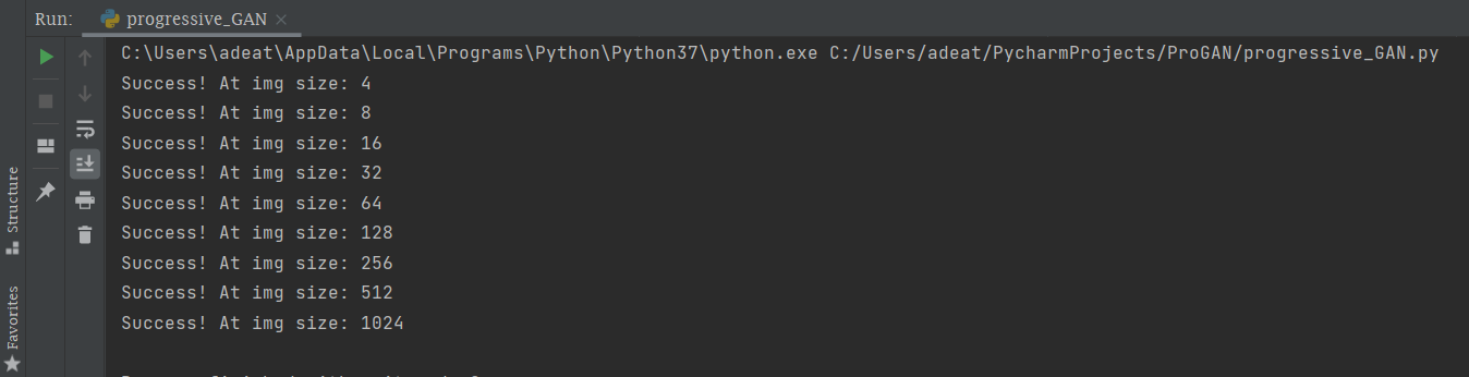
In the above code we all know about convolutional layers, generator, and discriminator, let us know what is pixel norm and mini-batch std.
Pixel norm and Mini Batch std:
Batch Normalization is not used here, instead of that two other techniques are introduced here, including pixel-wise normalization and minibatch standard deviation.
A pixel-wise normalization process is mainly performed in the generator after each convolutional layer which normalizes each pixel value in the activation map across the channels to a unit length. This is more generally referred to as “local response normalization.”
The standard deviation of activation function across the images in the mini-batch is added as a new channel which is prior to the last block of convolutional layers in the discriminator model. This is referred to as “Minibatch standard deviation.”
Then we need a utility file to do the following: Create a python file named ‘utils’
– plot to tensorboard
– gradient penalty
– Save checkpoint
– Load checkpoint
– Generate Examples
The below code will do all these
import torch
import random
import numpy as np
import os
import torchvision
import config
from torchvision.utils import save_image
from scipy.stats import truncnorm
# Print losses occasionally and print to tensorboard
def plot_to_tensorboard(
writer, loss_critic, loss_gen, real, fake, tensorboard_step
):
writer.add_scalar("Loss Critic", loss_critic, global_step=tensorboard_step)

with torch.no_grad():
# take out (up to) 8 examples to plot
img_grid_real = torchvision.utils.make_grid(real[:8], normalize=True)
img_grid_fake = torchvision.utils.make_grid(fake[:8], normalize=True)
writer.add_image("Real", img_grid_real, global_step=tensorboard_step)
writer.add_image("Fake", img_grid_fake, global_step=tensorboard_step)


def gradient_penalty(critic, real, fake, alpha, train_step, device="cpu"):
BATCH_SIZE, C, H, W = real.shape
beta = torch.rand((BATCH_SIZE, 1, 1, 1)).repeat(1, C, H, W).to(device)
interpolated_images = real * beta + fake.detach() * (1 - beta)
interpolated_images.requires_grad_(True)

# Calculate critic scores
mixed_scores = critic(interpolated_images, alpha, train_step)

# Take the gradient of the scores with respect to the images
gradient = torch.autograd.grad(
inputs=interpolated_images,
outputs=mixed_scores,
grad_outputs=torch.ones_like(mixed_scores),
create_graph=True,
retain_graph=True,
)[0]
gradient = gradient.view(gradient.shape[0], -1)
gradient_norm = gradient.norm(2, dim=1)
gradient_penalty = torch.mean((gradient_norm - 1) ** 2)
return gradient_penalty


def save_checkpoint(model, optimizer, filename="my_checkpoint.pth.tar"):
print("=> Saving checkpoint")
checkpoint = {
"state_dict": model.state_dict(),
"optimizer": optimizer.state_dict(),
}
torch.save(checkpoint, filename)


def load_checkpoint(checkpoint_file, model, optimizer, lr):
print("=> Loading checkpoint")
checkpoint = torch.load(checkpoint_file, map_location="cuda")
model.load_state_dict(checkpoint["state_dict"])
optimizer.load_state_dict(checkpoint["optimizer"])

# If we don't do this then it will just have learning rate of old checkpoint
# and it will lead to many hours of debugging :
for param_group in optimizer.param_groups:
param_group["lr"] = lr

def generate_examples(gen, steps, truncation=0.7, n=100):
"""
 Tried using truncation trick here but not sure it actually helped anything, you can
 remove it if you like and just sample from torch.randn
 """
 gen.eval()
alpha = 1.0
for i in range(n):
with torch.no_grad():
noise = torch.tensor(truncnorm.rvs(-truncation, truncation, size=(1, config.Z_DIM, 1, 1)), device=config.DEVICE, dtype=torch.float32)
img = gen(noise, alpha, steps)
save_image(img*0.5+0.5, f"saved_examples/img_{i}.png")

gen.train()
In the above code ‘plot_to_tensorboard’ will plot the training progress to tensoboard, ‘save_checkpoint’ function will save the model after each poch and ‘load_checkpoint’ will load the model for evaluation and ‘generate_example’ will save the generated images.
Then we need a configuration file through which we can specify Image size, Dataset path, checkpoint paths, device, batch size, learning rate, number of steps, epochs, and number of workers. You can change the configurations according to your desired setup. so, create a python file named ‘config’.
The dataset used here is celeb_HQ from the kaggle
import torch
from math import log2
START_TRAIN_AT_IMG_SIZE = 256
DATASET = 'Dataset'
CHECKPOINT_GEN = "generator.pth"
CHECKPOINT_CRITIC = "discriminator.pth"
DEVICE = "cuda" if torch.cuda.is_available() else "cpu"
SAVE_MODEL = True
LOAD_MODEL = False
LEARNING_RATE = 1e-3
BATCH_SIZES = [32, 32, 32, 16, 16, 16, 16, 8, 4]
IMAGE_SIZE = 512
CHANNELS_IMG = 3
Z_DIM = 256 # should be 512 in original paper
IN_CHANNELS = 256 # should be 512 in original paper
CRITIC_ITERATIONS = 1
LAMBDA_GP = 10
NUM_STEPS = int(log2(IMAGE_SIZE / 4)) + 1

PROGRESSIVE_EPOCHS = [50] * len(BATCH_SIZES)
FIXED_NOISE = torch.randn(8, Z_DIM, 1, 1).to(DEVICE)
NUM_WORKERS = 4
Now let’s train the model
Create a python file with the name ‘train’ so that we can write progressive GAN training code. The below code is linked to all the above code files.
import torch
import torch.optim as optim
import torchvision.datasets as datasets
import torchvision.transforms as transforms
from torch.utils.data import DataLoader
from torch.utils.tensorboard import SummaryWriter
from utils import (
    gradient_penalty,
    plot_to_tensorboard,
    save_checkpoint,
    load_checkpoint,
    generate_examples
)
from progressive_GAN import Discriminator, Generator
from math import log2
from tqdm import tqdm
import config
torch.backends.cudnn.benchmarks = True


def get_loader(image_size):
transform = transforms.Compose(
[
transforms.Resize((image_size, image_size)),
transforms.ToTensor(),
transforms.RandomHorizontalFlip(p=0.5),
transforms.Normalize(
[0.5 for _ in range(config.CHANNELS_IMG)],
[0.5 for _ in range(config.CHANNELS_IMG)],
),
]
)
batch_size = config.BATCH_SIZES[int(log2(image_size / 4))]
dataset = datasets.ImageFolder(root=config.DATASET, transform=transform)
loader = DataLoader(
dataset,
batch_size=batch_size,
shuffle=True,
num_workers=config.NUM_WORKERS,
pin_memory=True,
)
return loader, dataset


def train_fn(
critic,
gen,
loader,
dataset,
step,
alpha,
opt_critic,
opt_gen,
tensorboard_step,
writer,
scaler_gen,
scaler_critic,
):
loop = tqdm(loader, leave=True)
for batch_idx, (real, _) in enumerate(loop):
real = real.to(config.DEVICE)
cur_batch_size = real.shape[0]

# Train Critic: max E[critic(real)] - E[critic(fake)] <-> min -E[critic(real)] + E[critic(fake)]
# which is equivalent to minimizing the negative of the expression
noise = torch.randn(cur_batch_size, config.Z_DIM, 1, 1).to(config.DEVICE)

with torch.cuda.amp.autocast():
fake = gen(noise, alpha, step)
critic_real = critic(real, alpha, step)
critic_fake = critic(fake.detach(), alpha, step)
gp = gradient_penalty(critic, real, fake, alpha, step, device=config.DEVICE)
loss_critic = (
-(torch.mean(critic_real) - torch.mean(critic_fake))
+ config.LAMBDA_GP * gp
+ (0.001 * torch.mean(critic_real ** 2))
)

opt_critic.zero_grad()
scaler_critic.scale(loss_critic).backward()
scaler_critic.step(opt_critic)
scaler_critic.update()

# Train Generator: max E[critic(gen_fake)] <-> min -E[critic(gen_fake)]
with torch.cuda.amp.autocast():
gen_fake = critic(fake, alpha, step)
loss_gen = -torch.mean(gen_fake)

opt_gen.zero_grad()
scaler_gen.scale(loss_gen).backward()
scaler_gen.step(opt_gen)
scaler_gen.update()

# Update alpha and ensure less than 1
alpha += cur_batch_size / (
(config.PROGRESSIVE_EPOCHS[step] * 0.5) * len(dataset)
)
alpha = min(alpha, 1)

if batch_idx % 500 == 0:
with torch.no_grad():
fixed_fakes = gen(config.FIXED_NOISE, alpha, step) * 0.5 + 0.5
plot_to_tensorboard(
writer,
loss_critic.item(),
loss_gen.item(),
real.detach(),
fixed_fakes.detach(),
tensorboard_step,
)
tensorboard_step += 1

loop.set_postfix(
gp=gp.item(),
loss_critic=loss_critic.item(),
)

return tensorboard_step, alpha


def main():
gen = Generator(
config.Z_DIM, config.IN_CHANNELS, img_channels=config.CHANNELS_IMG
).to(config.DEVICE)
critic = Discriminator(
config.Z_DIM, config.IN_CHANNELS, img_channels=config.CHANNELS_IMG
).to(config.DEVICE)

# initialize optimizers and scalers for FP16 training
opt_gen = optim.Adam(gen.parameters(), lr=config.LEARNING_RATE, betas=(0.0, 0.99))
opt_critic = optim.Adam(
critic.parameters(), lr=config.LEARNING_RATE, betas=(0.0, 0.99)
)
scaler_critic = torch.cuda.amp.GradScaler()
scaler_gen = torch.cuda.amp.GradScaler()

# for tensorboard plotting
writer = SummaryWriter(f"logs/gan1")

if config.LOAD_MODEL:
load_checkpoint(
config.CHECKPOINT_GEN, gen, opt_gen, config.LEARNING_RATE,
)
load_checkpoint(
config.CHECKPOINT_CRITIC, critic, opt_critic, config.LEARNING_RATE,
)

gen.train()
critic.train()

tensorboard_step = 0
# start at step that corresponds to img size that we set in config
step = int(log2(config.START_TRAIN_AT_IMG_SIZE / 4))
for num_epochs in config.PROGRESSIVE_EPOCHS[step:]:
alpha = 1e-5 # start with very low alpha
loader, dataset = get_loader(4 * 2 ** step) # 4->0, 8->1, 16->2, 32->3, 64 -> 4
print(f"Current image size: {4 * 2 ** step}")

for epoch in range(num_epochs):
print(f"Epoch [{epoch+1}/{num_epochs}]")
tensorboard_step, alpha = train_fn(
critic,
gen,
loader,
dataset,
step,
alpha,
opt_critic,
opt_gen,
tensorboard_step,
writer,
scaler_gen,
scaler_critic,
)

if config.SAVE_MODEL:
save_checkpoint(gen, opt_gen, filename=config.CHECKPOINT_GEN)
save_checkpoint(critic, opt_critic, filename=config.CHECKPOINT_CRITIC)

step += 1 # progress to the next img size


if __name__ == "__main__":
main()
Once the code starts training you can check the training progress with the help of tensorboard
TensorBoard provides the tooling and visualization needed for machine learning experimentation:
– Tracking and visualizing metrics such as loss and accuracy
– Visualizing the model graph (ops and layers)
– Viewing histograms of weights, biases, or other tensors as they change over time
– Projecting embeddings to a lower-dimensional space
– Displaying images, text,
and audio data
just run the below command in your project directory with help of the command window(CMD) to track the training process.
tensorboard --logdir logs
This will generate a link, copy that link and paste it in the browser, tensoboard dashboard will be opened.
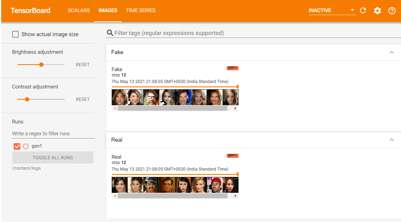
Here you can track the training progress and also can see the generated fake images.
The code is available in the below GitHub link
For more information about Progressive GAN refer to the official paper
https://arxiv.org/abs/1710.10196
Hope you enjoyed training ProGAN.
The media shown in this article are not owned by Analytics Vidhya and is used at the Author’s discretion.
I thrive on the thrill of the challenge, tackling complex problems and crafting innovative AI solutions that make a difference. Whether it's optimizing or building sustainable AI ecosystems, I believe in harnessing the power of AI for the greater good. Let's brainstorm, collaborate, and change the world, one byte at a time.


Thanks a lot for such a good article and useful code! You wrote: The code is available in the below GitHub link. But the link itself is missing in the text of the article.