Artificial Neural Networks – Better Understanding !

Introduction

Artificial Neural Networks (ANN)are the basic algorithms and also simplified methods used in Deep Learning (DL) approach. We have come across more complicated and high-end models in the DL approach. However, ANN is a vital element of the progressive procedure and is the first stage in the DL algorithm.

Before wetting our hands over ANN, we have to comprehend the importance or existence of DL. ANN is established by the human brain activity, therefore our neural system can be understood by ANN as a way of transmitting our information via neurons to our brain. Thus, through some significant layman terms, we shall learn about ANN in forthcoming topics.

In this article you will get understanding about the artificial neural networks and how these ann works, and these ann code is implementing in these areas and also we are provding the concept of Neuron to form as Artificial Neural Networks.

This article was published as a part of the Data Science Blogathon

Neuron – Concept Introduction to form as ANN:

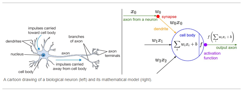
In our school time, most of them find this diagram. In simple terms, the fundamental job of the neuron is to receive and transmit impulses/information in various parts of our own body. In a simple, neuron which forges building blocks of our human nervous system. By the way, there will be no single neuron, the building block generates millions and millions of neurons. Just think of the circumstance as a car accident happened in front of our flat, what our brain will think immediately, go for help if feasible to seek assistance, if not contacting the ambulance.

Here, while we have seen so many neuronal elements, Dendrites are regarded as a signal receiver and Axon as a signal transmitter. In this figure, to better understand, it shows a signal from a neuron that passes along its axon and links or transmits to dendrites of another neuron (Axon is not technically touched dendrites of another neuron, the process is called Synapse for receiving and transmitting the signals). What if the concepts mentioned above are artificial? What if? Artificial Neural Network’s name comes there!

Neural Network – Basic foundation to understand:

Now biological notions, as demonstrated in the previous subject, become a technological approach in this graphical representation above. So let’s assume, x1, x2…xn is considered as multiple neurons (presumed to be multiple sensory) transmitting signal to a signal neuron. Let us assume a scenario for the above diagram, you are going to watch a horror movie with your friends in a theatre, so there is a particular scene where the whole theatre gets erupted for a horror scene and you are having horror phobia (fear of watching horror scene), so for that scene what you do? assume x1 – eyes, x2 – ears, and x3 – mouth are some of the inputs, then what about your outputs be like? You will automatically close your eyes, close your ears and scream more (as like the voice in the movie is not audible) as per the scenario. In short, it can be picturized as,

We have terms like w1, w2, w3 which means weights: Weights are crucial for ANN function because weights are how neural networks (NN) learn, by modifying the weights, the NN decides which signal is significant in each case and which signal is not relevant for neurons, or which signal is passed or which signal is not passed or to which intensity signal is passed, they are the things that can be adapted through the learning method, like when you are training ANN, you are basically adjusting all the weights, and that’s where Gradient
Descent (GD) and Back Propagation (BP) comes into play, so for the same scenario, you will be having the priority right which part has the highest weightage to process – here by default we close our eyes right. Finally, the dotted line (blue lines) here in the above diagram means Synapse, communication
between neurons.

To summarize in short, how neural network takes place

1. Signals from multiple neurons like x1, x2, x3… xn, along with associated weights w1, w2, w3… wn are transmitted to the successive neurons. (Input layers)

2. So after we are receiving multiple signals (here consider it as neurons), with weights associated with it, we will be summing up all the signals with weights, and that’s our step 1 as shown in the above figure (Hidden layers).

3. Then it applies the activation function as step 2 as shown in the above figure (Hidden layers).

4. From the above step neuron understand if it needs to pass the signal or not.

5. If the neuron passes the signal (that’s to another neuron), that’s our output (Output layers).

6. The above process keeps on repeating until the last neuron or the part of our body here.

Finally, NN is a sequence of algorithms that imitate human brain functions to recognize connections between huge volumes of data. This is the basis for the DL approach, and NN can be categorized as stated below based on the architecture,

What is the Activation Function? – Superpower for Artificial Neural Networks

So what actually Activation Function (AF) do? AF is a function that is added into an ANN to help the network learn complex patterns in the data. When comparing with a neuron-based model that is in our brains, the activation function is at the end deciding what is to be fired to the next neuron. It takes in the output signal from the previous cell and converts it into some form that can be taken as input to the next cell. It’s a non-linear transformation that we do for inputs that we receive before sending them to the next layer or neuron. AF is also known as Transfer Function.

So basically AF can be classified into linear AF and non-linear AF. In simple, without AF, the output signal will be a linear function (like polynomial of one degree or as a linear regression model) – they have less power to learn the complex functional mapping from data. AF captures a non-linear relationship between the inputs and also converts the inputs to useful output.

But our brain functions non-linearly for complex calculation, robustness, and high parallelism, ability to handle imprecise and fuzzy information. So for this to mimic we need AF, to work in the complicated, high dimensional, and non-linear large dataset that has complicated architecture (having many hidden layers between input and output layers).

To understand the non-linear Af, we need to understand two terminologies like,

1. Differential function: Change in Y-axis w.r.t change in X-axis (slope!)

2. Monotonic function: A function which either entirely non decreasing or non increasing. (Non-linear!)

Some important key features for AF,

1. Vanishing Gradient problem
2. Zero-Centered
3. Computational inexpensive
4. Differentiable

There are some important types of the non-linear activation function (classified based on curves),

Sigmoid function

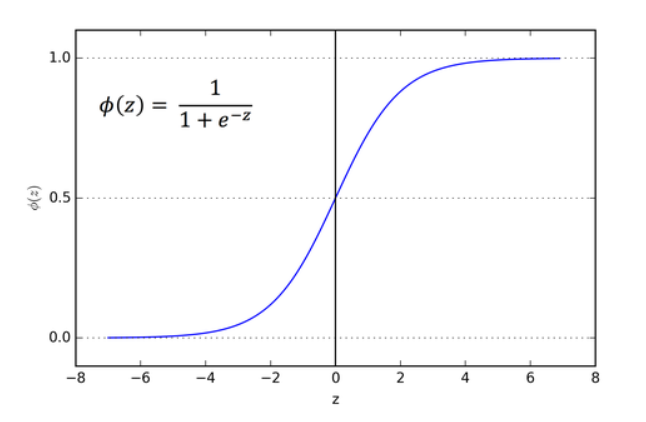
Bullet points for sigmoid function,

1. Zero is the threshold function here, if it is less than zero, then it passes to zero, if it is equal to zero or greater than zero then, it passes to one, as simple.

2. Application: Predominately used for binary classification

3. Its differentiable means we can find the slope at any two points

4. It is a monotonic function

5. Mostly won’t be used in real-world examples, because of computationally inexpensive, causes vanishing gradient problems, and not zero-centered.

Hyperbolic Tangent function (Tanh)

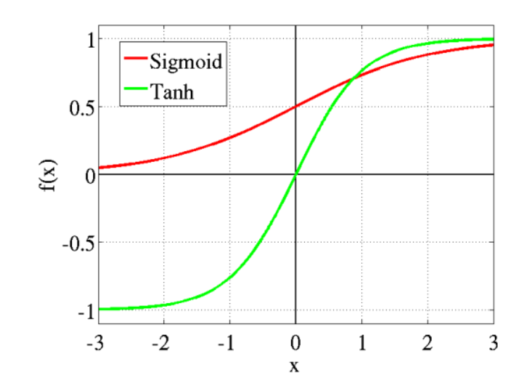
Bullet points for Hyperbolic Tangent function,

1. Better version of Sigmoid function (range: -1 to +1), goes below zero. 

2. It is a differentiable function

3. It is a monotonic function

4. Application: Used for two-class problems, Used in feedforward nets.

Softmax function

Bullet points for softmax function, 

1. This particular AF works in the output layer

2. Need to apply a standard exponential function to all the values in the output layer, then do the normalization by dividing the sum of all exponentials. (Sum of all makes to 1)

3. Application: Multi-class classification problems (confidence score for each class)

4. It is a differentiable function

Rectified Linear Unit (ReLU) function

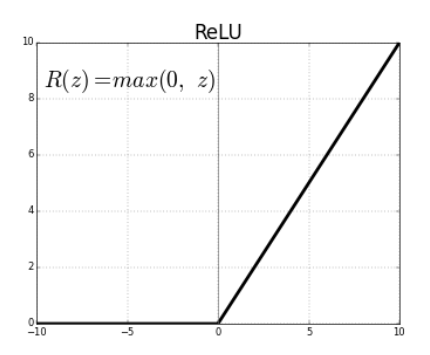
Bullet points for Rectifier Linear Unit (ReLU) function,

1. Most used in CNN and many DL approaches because does not cause vanishing gradient problem.

2. If the value is less than zero, then the function becomes zero, if the value is equal to zero or greater than the function becomes the number. – dying ReLU (which causes some nodes to completely die and not learn anything)

3. It is a differentiable function

4. It is not a monotonic function

5. Range of this AF is o to infinity

6. Disadvantage: If any value is less than zero then automatically function makes it to zero, which makes the negative value not mapped properly except but zero and also leads to the unstable node.  

Leaky ReLU

Bullet points for Leaky Rectifier Linear Unit function,

1. Advance function of ReLU, and it solves negative impact of ReLU function

2. Usually the “a” value in the above diagram is around 0.01 only, if it exceeds means it became Randomized ReLU (mostly we stick with ReLU and sometimes with Leaky ReLU AF only)

3. Range of Leaky ReLU is – infinity to + infinity

4. It is a differentiable function

5. It is a monotonic function

Exponential Linear Units (ELUs) function 

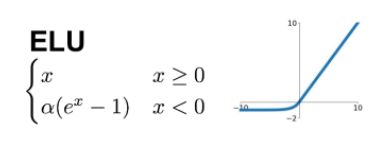
Bullet points for Exponential Linear Unit function,

1. Advance to ReLU and Leaky ReLU AF

2. Because of the negative impact of the above-mentioned AFs, it causes mean unit activation greater than zero, hence it rectifies this, ELU AF comes to the picture and makes mean activation closer to zero, hence it makes the model faster learning and convergence

3. It is a differentiable function

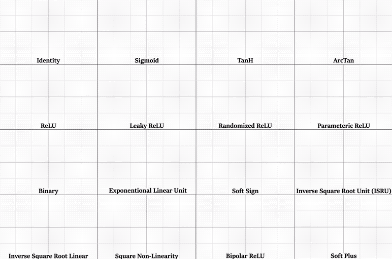
and some other AF are picturized below,

Note: Among all, Tanh and Sigmoid AF can’t be used more in real-time because of vanishing gradient problems. 

How NN learn? – Some interesting topics ALERT!

Before getting into the topic, we must know about two basic terminologies like Feed-forward and Back Propagation network. In simple term,

1. Feed Forward network (FFN) – If we achieved output what we expected from the input without turning back or fine-tuning.

2. Back Propagation Network (BPN) – Opposite to FFN, if the output that we got is not as expected and we need to turn back for fine-tuning it to the expected output. (learning and adjusting!)

So here in this picture, don’t see the residual concept, consider only actual and predicted values alone, here there will be two scenarios,

1. If the predicted output equals actual output then no worries.

2. If the predicted output varies with actual output, then we need to find the difference between the outputs, which we call as COST (error) function, our main goal is to reduce it. So we go for BPN (weights get updated and then proceed until cost function is reduced but not zero!)

Gradient Descent:

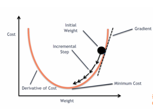
Let’s assume that we have a data set with fewer characteristics (independent variables), it is very obvious from the figure above that when we generate series of cost values, and we can find the least-cost value in a
simple model while updating different weights. If our dataset has more characteristics or separate variables, we must suffer a curse of dimensionality (CoD).

As the dimentionality of the features space increases, the number of configurations can grow exponentially and thus the number of configurations covered by an observation increases.

The above picture, which explains the layman concept about CoD.

So according to Huges Phenomenon (below diagram), the curse of dimensionality, if the features are added, the accuracy of the classification model is increased until the ideal number of features are achieved and the accuracy is further diminished

So let us consider a neural network model with more number hidden layers and independent features as shown below or even greater than that, obviously, we will face CoD. So for this problem, one of the solutions is Gradient Descent

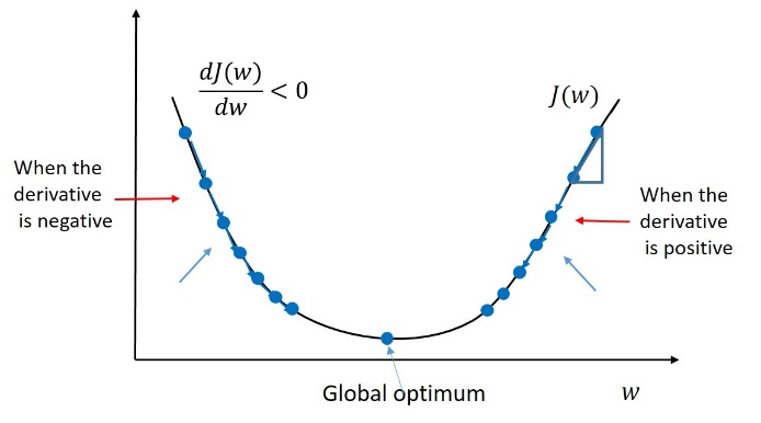
So let’s presume how GD works? Consider this is the cost function of our model and blue dot which implies different iterations (here different weights adjustment), we will get different cost functions. We start from the left side first, for the top value let’s take the slope value, the value may be positive or negative irrespective of the values (numbers), if our value is negative then we need to move towards the downside, the same way in the right side top value again if we calculate the slope, if we get the negative value again move downwards or else upwards, so likewise we need to find out for all the values. Finally when we find the minimum value (best weights probably!) among all others is our minimum cost value function.

Limitation: Convex cost function (depends on the shape from cost values)

Gradient Descent = Descending into Minimum of COST function 

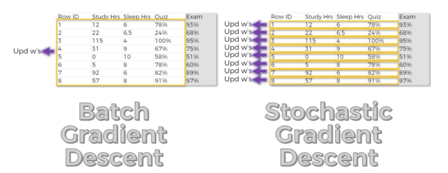
Stochastic Gradient Descent:

The main drawback of GD is limited to convex function (shape). Suppose for our dataset, while calculating cost function and then the shape of the cost function assume as like below picture, in that scenario can we proceed with same GD, the simple answer is no!, because if you note in the same figure, we have multiple minimum values (local minimum values), rather than the optimal value (global minimum), for this situation we opt for stochastic gradient descent optimization technique (SGD).

The only difference between GD and SGD are,

1. In GD, we will take all rows (here samples we call), plug them into our network model, then find the output value and then correlate with actual value, find the cost function, then revert (by backpropagation network) adjust the weights and proceed further for different values among them, we will find the minimum values of the cost function.

2. In SGD, we follow the same steps as GD only one difference is instead of applying all samples we go for each row separately and update the weights.

For more clarification between GD and SGD, find out the below picture,

Mini Batch Gradient Descent = Gradient Descent + Stochastic Gradient Descent

Back Propagation:

As we know, BPN means after finding the output value, we are going to compare with the actual value, then we will find the errors, after that to minimize the error, we are backpropagated then do some adjustments with weights then again we proceed until we get the minimum error. BPN is an advanced algorithm, which has more complex mathematics for adjusting weights simultaneously. The main advantage of BPN is the way the algorithm is structured because we can adjust the weights simultaneously and also basically we know which part of the NN which is part of the weight is responsible for the error.

How network works? – Overall Summary!

Bullet points on how NN works in general,

1. the First layer is the input layer as we all know.

2. the Last layer is the output layer that’s by default.

3. Assume here we don’t have a hidden layer, we need to calculate the price of the house, and let’s consider the inputs are area, no. of bedrooms, distance from the city, amenities available, age of the property, hospitals and schools for kids, so the price will be simply the summation of the product between input’s and weightage priority and with AF we will calculate the price. So it’s almost like a Machine learning model.

4. So what makes DL approach something better than the Machine Learning model is the addition of a hidden layer, it gives some flexibility and power, to increase accuracy.

5. Let us consider, for the same example above all the inputs are connected to all the neurons in the hidden layer, which means it won’t have the same weightage from the input layer, which means depending on the priorities the weightage values changes (Higher priority have high values!) Ex: We all know the flat rate is more in the city rather than the flat rate in outer of the city for the same square feet likewise it changes with other inputs as we mentioned. Each neuron in the hidden layer has some priorities and weightage for application-related like how our brain works?

6. If we keep on increasing the hidden layers for some importance or weightage or for solving complex calculations, the accuracy gets increased, it’s like fine-tuning the network to get the optimal output.

7. We will be using two AF for a simpler NN, i.e, 1st between input and hidden layer, 2nd between hidden and output layer.

The below picture summarizes the whole concept,  here let us assume the inputs x1, x2 be the study hours, sleeping hours, and quizzes, so with weightage given it is passed to the hidden layer and it performs the summation and by applying AF, we get the output values. then it is compared with the actual value, if the error value is more, that we call it a cost function then again it was backpropagated then adjusted the weight, then again process continued until we get minimal cost value, and the optimization process is called gradient descent, if the whole samples (rows) processed and updating the weights or Stochastic gradient descent if each row is processed and updates it’s the weight (mostly we will be using this because of it’s robust nature)

The below steps which summarize all,

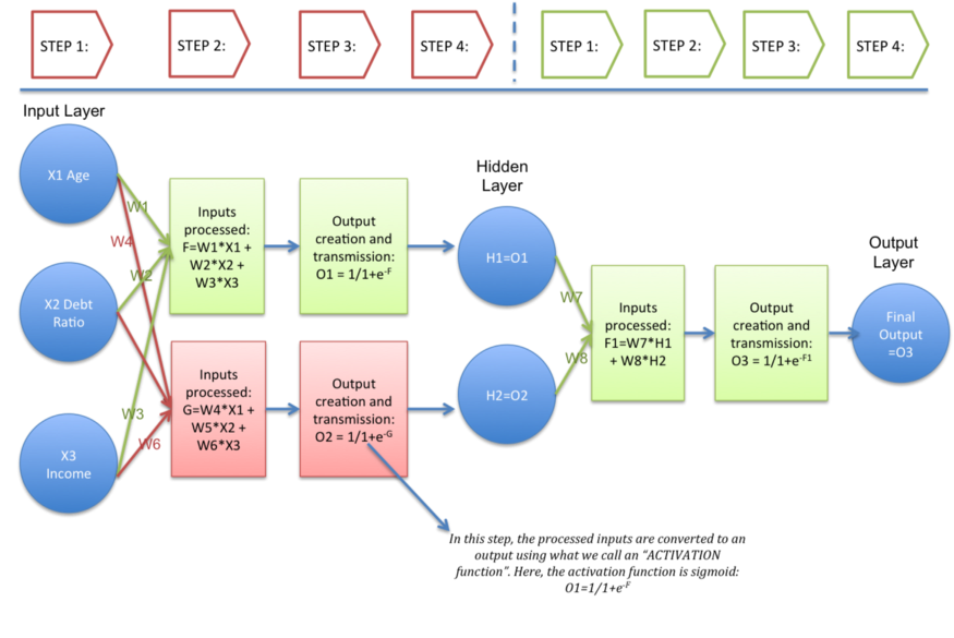
Overall, ANN can be picturized in general as,

Advantage: 

1. Ability to work with incomplete knowledge

2. Fault tolerance

3. Parallel processing capability

Disadvantage: 

1. Hardware dependence

2. Duration of the network is unknown

Application:

1. Handwritten Recognition

2. Image compression

3. Stock exchange prediction

I hope now understand how ANN works theoretically, let’s understand more through my Python coding,

Classification Part

Dataset: https://www.kaggle.com/shrutimechlearn/churn-modelling

In the first step, we are going to importing the basic libraries needed for ANN

#import libraries
import numpy as np
import pandas as pd
import tensorflow as tf

In the next step, we are going to import the dataset

#importing dataset
dataset = pd.read_csv('Churn_Modelling.csv')

Before modeling, we need to analyze the dataset for that first need to view the data for the partial outlook

import pandas as pd

#importing dataset
dataset = pd.read_csv('Churn_Modelling.csv')

#partial view of dataset from top
print(dataset.head())

#partial view of dataset from bottom
print(dataset.tail())

#basic dataset information
print(dataset.info())

#dimension of the dataset
print(dataset.shape)

#basic statistics summary
print(dataset.describe().T)

import pandas as pd

#importing dataset
dataset = pd.read_csv('Churn_Modelling.csv')

#partial view of dataset from top
print(dataset.head())

#partial view of dataset from bottom
print(dataset.tail())

#basic dataset information
print(dataset.info())

#dimension of the dataset
print(dataset.shape)

#basic statistics summary
print(dataset.describe().T)

next for checking missing values

#checking for missing values
print(str('Any missing data or NaN in the dataset:'),dataset.isnull().values.any())

next is finding the correlation between features

#finding correlation between the features
corr_var=dataset.corr()
print(corr_var)
plt.figure(figsize=(10,7.5))
sns.heatmap(corr_var, annot=True, cmap='BuPu')

X = dataset.iloc[:, 3:-1].values

#target value

y = dataset.iloc[:, -1].values

#as we have two columns as categorical terms we go for encoding we need to convert to numericals
#Categorical encoding
#gender will have some correlation with other feature so we go for label encoding
from sklearn.preprocessing import LabelEncoder
le = LabelEncoder()
#gender column in index 2
X[:, 2] = le.fit_transform(X[:, 2])

#country name wont be that much correlation added it has more than 2 names so go for one hot encoding
from sklearn.compose import ColumnTransformer
from sklearn.preprocessing import OneHotEncoder
#country name is present in 1st index value
ct = ColumnTransformer(transformers=[('encoder', OneHotEncoder(), [1])], remainder='passthrough')
X = np.array(ct.fit_transform(X))

#training and testing split
from sklearn.model_selection import train_test_split
X_train, X_test, y_train, y_test = train_test_split(X, y, test_size = 0.3, random_state = 0)

#feature scaling is an important and mandatory for ann process before modelling
from sklearn.preprocessing import StandardScaler
sc = StandardScaler()
X_train = sc.fit_transform(X_train)
X_test = sc.transform(X_test)

#ANN - initializing
ann = tf.keras.models.Sequential()

#input layer
# 6 features
ann.add(tf.keras.layers.Dense(units=6, activation='relu'))

#hidden layer
ann.add(tf.keras.layers.Dense(units=6, activation='relu'))

#output layer
#as target value is binary - AF
ann.add(tf.keras.layers.Dense(units=1, activation='sigmoid'))

#compiling
#loss - target is binary 
ann.compile(optimizer = 'adam', loss = 'binary_crossentropy', metrics = ['accuracy'])

#training set
ann.fit(X_train, y_train, batch_size = 32, epochs = 50)

<div>
<div>
<pre><span style="font-size: 12.25px;">#test result - prediction</span></pre>
<pre>y_pred = ann.predict(X_test)</pre>
</div>
</div>

#insted of values we ll get 0 or 1
y_pred = (y_pred > 0.5)
#actual vs prediicted outputs
print(np.concatenate((y_pred.reshape(len(y_pred),1), y_test.reshape(len(y_test),1)),1))

#accuracy and confusion matrix

from sklearn.metrics import confusion_matrix, accuracy_score
cm = confusion_matrix(y_test, y_pred)
print(cm)
accuracy_score(y_test, y_pred)

[[2276  103]

[ 310  311]]

0.8623333333333333

For full python coding and the output visit my page:

EndNote:

In this article, we have discussed Artificial Neural Networks from the working of neuron, what is a neural network, activation function and its types, then how neural network learns, gradient descent, stochastic gradient descent, backpropagation, a summary of ANN, advantage, and disadvantage then lastly application of ANN. In the last session, I have included Python code for ANN step by step for a simple dataset, by doing the slight modification, we can adopt this coding for all types of dataset.

Hope you like the article and get understanding about the artificial neural networks, Now you how these ANN concept in neuron and with these artificial neural networks you have also help for coding and clear insights in sigmoid function and activation function in artificial neural networks.

Did you find this article helpful? Please share your opinions/thoughts in the comments section below. Learn from mistakes is my favorite quote, if you found anything wrong too, just highlight it, I am ready to learn from the learners like you people.

To gain a deeper understanding and practical insights, explore the detailed explanation of the working of neural networks and elevate your knowledge to the next level!

The media shown in this article are not owned by Analytics Vidhya and are used at the Author’s discretion.

Premanand S

Premanand S is a dedicated academic with over a decade of research experience, specializing in Bio-signal Processing, Machine Learning, and Deep Learning. He completed his B.Tech in 2009 from Amrita Vishwa Vidyapeetham, Bangalore, and his M.E. in 2011 from Rajalakshmi Engineering College, Chennai, where his thesis focused on Deep Learning for ECG Signal Processing.

He is pursuing his Ph.D. at VIT-Chennai, with a tentative research title of "Deep Learning Approaches for Enhanced ECG Signal Processing and Arrhythmia Classification." His research aims to leverage cutting-edge deep learning techniques to improve the accuracy and efficiency of ECG signal analysis, contributing significantly to cardiac health monitoring.

A recipient of the prestigious TCS-RSP (Research Scholarship) in 2014, Cycle 9, Premanand has become a recognized figure in the academic community. He has delivered several invited talks on Data Science, Machine Learning, and Deep Learning at prominent institutions across India.

In his role as an Assistant Professor at VIT-Chennai, he continues to inspire the next generation of researchers while advancing the boundaries of knowledge in his field.