Flight Price Prediction -A Regression Analysis using Lazy Prediction

This article was published as a part of the Data Science Blogathon

This Blog deals with the problem of flight price prediction.

1. Objective

The objective of this article is to predict flight prices given the various parameters. Data used in this article is publicly available at Kaggle. This will be a regression problem since the target or dependent variable is the price (continuous numeric value).

2. Introduction

Airline companies use complex algorithms to calculate flight prices given various conditions present at that particular time. These methods take financial, marketing, and various social factors into account to predict flight prices.

Nowadays, the number of people using flights has increased significantly. It is difficult for airlines to maintain prices since prices change dynamically due to different conditions. That’s why we will try to use machine learning to solve this problem. This can help airlines by predicting what prices they can maintain. It can also help customers to predict future flight prices and plan their journey accordingly.

3. Data Used

Data was used from Kaggle which is a freely available platform for data scientists and machine learning enthusiasts.

Source: https://www.kaggle.com/nikhilmittal/flight-fare-prediction-mh

We are using jupyter-notebook to run Flight Price Prediction task.

4. Data Analysis

The procedure of extracting information from given raw data is called data analysis. Here we will use eda module of data-prep library to do this step.

from dataprep.eda import create_report
import pandas as pd
dataframe = pd.read_excel("../output/Data_Train.xlsx")
create_report(dataframe)

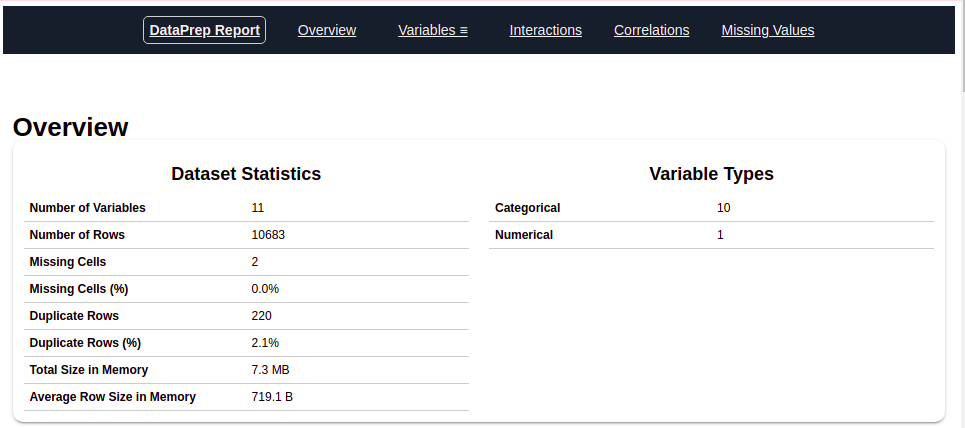
After running the above code you will get a report as shown in the above figure. This report contains various sections or tabs.  ‘Overview’ section of this report provides us with all the basic information of the data we are using. For the current data we are using we got the following information:

Number of variables = 11
Number of rows = 10683
Number of categorical type of feature = 10
Number of numerical type of feature = 1
Nuplicate rows = 220 e.t.c

Let’s explore other sections of the report one by one.

4.1 Variables

After you select the variable section you will get information as shown in the below figures.

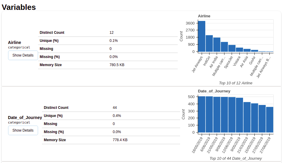
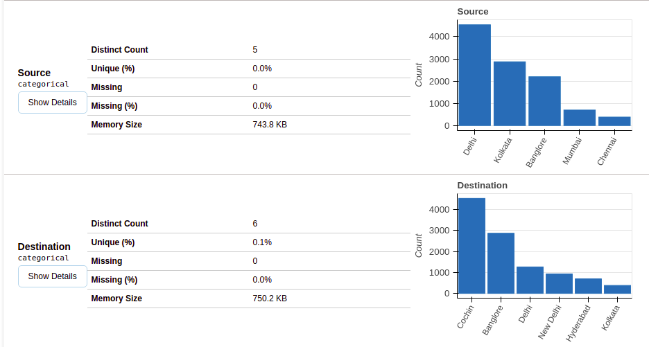
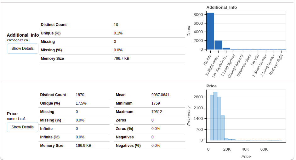
This section provides the type of each variable along with a detailed description of the variable.

4.2 Missing Values

This section has multiple ways using which we can analyze missing values in variables. We will discuss three mostly used methods, bar-chart, spectrum, and Heat Map. Let’s explore each one by one.

4.2.1 Bar Chart

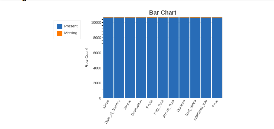
The bar chart method shows the ‘number of missing and present values’ in each variable in a different color.

4.2.2 Spectrum

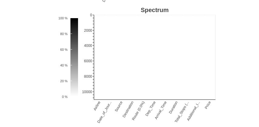
The spectrum method shows the percentage of missing values in each variable.

4.2.3 Heat Map

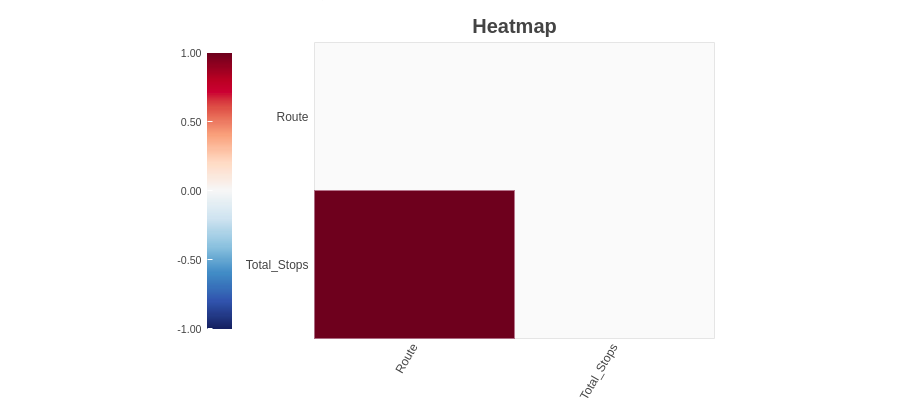
The heat Map method shows variables having missing values in terms of correlation. Since ‘Route’ and ‘Total_Stops’ both are highly correlated, they both have missing values.

As we can observe ‘Route’ and ‘Total_Stops’ variables have missing values. Since we did not find any missing values information from Bar-Chart and Spectrum method but we found missing value variables using the Heat Map method. Combining both of these information, we can say that the ‘Route’ and ‘Total_Stops’ variables have missing values but are very low.

5. Data Preparation

Before starting data preparation let’s have a glimpse of data first.

dataframe.head()

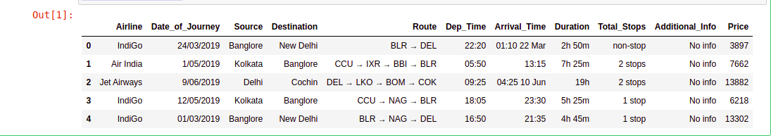
As we saw in Data Analysis there are 11 variables in the given data. Below is the description of each variable.

Airline: Name of the airline used for traveling

Date_of_Journey: Date at which a person traveled

Source: Starting location of flight

Destination: Ending location of flight

Route: This contains information on starting and ending location of the journey in the standard format used by airlines.

Dep_Time: Departure time of flight from starting location

Arrival_Time: Arrival time of flight at destination

Duration: Duration of flight in hours/minutes

Total_Stops: Number of total stops flight took before landing at the destination.

Additional_Info: Shown any additional information about a flight

Price: Price of the flight

Few observations about some of the variables:

1. ‘Price‘ will be our dependent variable and all remaining variables can be used as independent variables.

2. ‘Total_Stops‘ can be used to determine if the flight was direct or connecting.

5.1 Handling Missing Values

As we found out the ‘Route’ and ‘Total_Stops’ variables have very low missing values in data. Let’s now see the percentage of missing values in data.

(dataframe.isnull().sum()/dataframe.shape[0])*100

Output :

Airline            0.000000
Date_of_Journey    0.000000
Source             0.000000
Destination        0.000000
Route              0.009361
Dep_Time           0.000000
Arrival_Time       0.000000
Duration           0.000000
Total_Stops        0.009361
Additional_Info    0.000000
Price              0.000000
dtype: float64

As we can observe ‘Route’ and ‘Total_Stops’ both have 0.0094% of missing values. In this case, it is better to drop missing values.

dataframe.dropna(inplace= True)
dataframe.isnull().sum()

Output :

Airline            0
Date_of_Journey    0
Source             0
Destination        0
Route              0
Dep_Time           0
Arrival_Time       0
Duration           0
Total_Stops        0
Additional_Info    0
Price              0
dtype: int64

Now we don’t have any missing values.

5.2 Handling Date and Time Variables

We have ‘Date_of_Journey’, a ‘date type variable and ‘Dep_Time’, ‘Arrival_Time’ that captures time information.

We can extract ‘Journey_day’ and ‘Journey_Month’ from the ‘Date_of_Journey’ variable. ‘Journey day’ shows the day of the month on which the journey was started.

dataframe["Journey_day"] = pd.to_datetime(dataframe.Date_of_Journey, format="%d/%m/%Y").dt.day
dataframe["Journey_month"] = pd.to_datetime(dataframe["Date_of_Journey"], format = "%d/%m/%Y").dt.month
dataframe.drop(["Date_of_Journey"], axis = 1, inplace = True)

Similarly, we can extract ‘Departure_Hour’ and ‘Departure_Minute’ as well as ‘Arrival_Hour and ‘Arrival_Minute’ from ‘Dep_Time’ and ‘Arrival_Time’ variables respectively.

dataframe["Dep_hour"] = pd.to_datetime(dataframe["Dep_Time"]).dt.hour
dataframe["Dep_min"] = pd.to_datetime(dataframe["Dep_Time"]).dt.minute
dataframe.drop(["Dep_Time"], axis = 1, inplace = True)

dataframe["Arrival_hour"] = pd.to_datetime(dataframe.Arrival_Time).dt.hour
dataframe["Arrival_min"] = pd.to_datetime(dataframe.Arrival_Time).dt.minute
dataframe.drop(["Arrival_Time"], axis = 1, inplace = True)

We also have duration information on the ‘Duration’ variable. This variable contains both duration hours and minutes information combined.

We can extract ‘Duration_hours’ and ‘Duration_minutes’ separately from the ‘Duration’ variable.

def get_duration(x):
    x=x.split(' ')
    hours=0
    mins=0
    if len(x)==1:
        x=x[0]
        if x[-1]=='h':
            hours=int(x[:-1])
        else:
            mins=int(x[:-1])
    else:
        hours=int(x[0][:-1])
        mins=int(x[1][:-1])
    return hours,mins
dataframe['Duration_hours']=dataframe.Duration.apply(lambda x:get_duration(x)[0])
dataframe['Duration_mins']=dataframe.Duration.apply(lambda x:get_duration(x)[1])
dataframe.drop(["Duration"], axis = 1, inplace = True)

5.3 Handling Categorical Data

Airline, Source, Destination, Route, Total_Stops, Additional_info are the categorical variables we have in our data. Let’s handle each one by one.

Airline Variable

Let’s see how the Airline variable is related to the Price variable.

import seaborn as sns
sns.set()
sns.catplot(y = "Price", x = "Airline", data = train_data.sort_values("Price", ascending = False), kind="boxen", height = 6, aspect = 3)
plt.show()

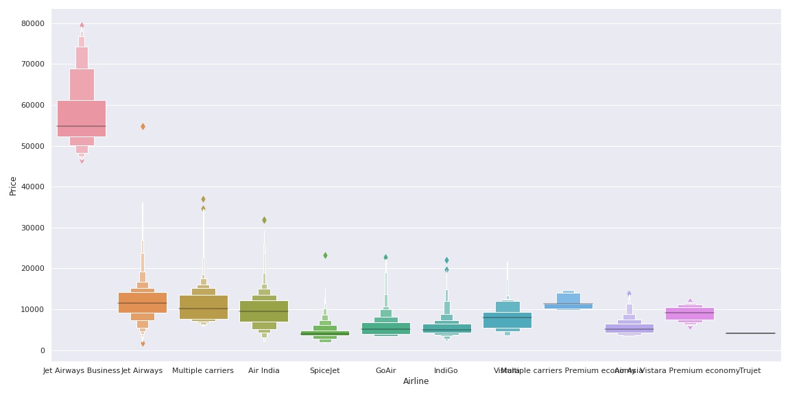
As we can see the name of the airline matters. ‘JetAirways Business’ has the highest price range. Other airlines price also varies.

Since the Airline variable is Nominal Categorical Data (There is no order of any kind in airline names) we will use one-hot encoding to handle this variable.

Airline = dataframe[["Airline"]]
Airline = pd.get_dummies(Airline, drop_first= True)

One-Hot encoded ‘Airline’ data is saved in the Airline variable as shown in the above code.

Source  and Destination Variable

Again ‘Source’ and ‘Destination’ variables are Nominal Categorical Data. We will use One-Hot encoding again to handle these two variables.

Source = dataframe[["Source"]]
Source = pd.get_dummies(Source, drop_first= True)
Destination = train_data[["Destination"]]
Destination = pd.get_dummies(Destination, drop_first = True)

Route variable

Route variable represents the path of the journey. Since the ‘Total_Stops’ variable captures the information if the flight is direct or connected so I have decided to drop this variable.

dataframe.drop(["Route", "Additional_Info"], axis = 1, inplace = True)

Total_Stops Variable

dataframe["Total_Stops"].unique()

Output:

array(['non-stop', '2 stops', '1 stop', '3 stops', '4 stops'],
      dtype=object)

Here, non-stop means 0 stops which means direct flight. Similarly meaning other values is obvious. We can see it is an Ordinal Categorical Data so we will use LabelEncoder here to handle this variable.

dataframe.replace({"non-stop": 0, "1 stop": 1, "2 stops": 2, "3 stops": 3, "4 stops": 4}, inplace = True)

Additional_Info variable

dataframe.Additional_Info.unique()

Output:

array(['No info', 'In-flight meal not included',
       'No check-in baggage included', '1 Short layover', 'No Info',
       '1 Long layover', 'Change airports', 'Business class',
       'Red-eye flight', '2 Long layover'], dtype=object)

As we can see, this feature captures relevant that can affect flight price significantly. Also ‘ No Info’ values are repeated. Let’s handle that first.

dataframe['Additional_Info'].replace({"No info": 'No Info'}, inplace = True)

Now this variable is also Nominal Categorical Data. Let’s use One-Hot Encoding to handle this variable.

Add_info = dataframe[["Additional_Info"]]
Add_info = pd.get_dummies(Add_info, drop_first = True)

5.4 Final Dataframe

Now we will create the final dataframe by concatenating all the One-hot and Label-encoded features to the original dataframe. We will also remove original variables using which we have prepared new encoded variables.

dataframe = pd.concat([dataframe, Airline, Source, Destination,Add_info], axis = 1)
dataframe.drop(["Airline", "Source", "Destination","Additional_Info"], axis = 1, inplace = True)

Let’s see the number of final variables we have in dataframe.

dataframe.shape[1]

Output:

38

So, we have 38 variables in the final dataframe including the dependent variable ‘Price’. There are only 37 variables for training.

6. Model Building

X=dataframe.drop('Price',axis=1)
y=dataframe['Price']
#train-test split
from sklearn.model_selection import train_test_split
x_train, x_test, y_train, y_test = train_test_split(x, y, test_size = 0.2, random_state = 42)

6.1 Applying Lazy Prediction

One of the problems of the model-building exercise is ‘How to decide which machine learning algorithm to apply ?’

This is where Lazy Prediction comes into the picture. Lazy Prediction is a machine learning library available in python that can quickly provide us with performances of multiple standard classifications or regression models on multiple performance matrices.

Let’s see how it works…

Since we are working on a Regression task we will use Regressor models.

from lazypredict.Supervised import LazyRegressor
reg = LazyRegressor(verbose=0, ignore_warnings=False, custom_metric=None)
models, predictions = reg.fit(x_train, x_test, y_train, y_test)
models.head(10)

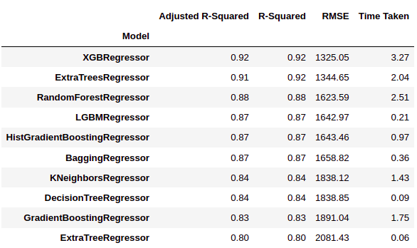
As we can see LazyPredict gives us results of multiple models on multiple performance matrices. In the above figure, we have shown the top ten models.

Here ‘XGBRegressor’ and ‘ExtraTreesRegressor’ outperform other models significantly. It does take a high amount of training time with respect to other models. At this step we can choose priority either we want ‘time’ or ‘performance’.

We have decided to choose ‘performance’ over training time. So we will train ‘XGBRegressor and visualize the final results.

6.2 Model Training

from xgboost import XGBRegressor
model =  XGBRegressor()
model.fit(x_train,y_train)

Output:

XGBRegressor(base_score=0.5, booster='gbtree', colsample_bylevel=1,
             colsample_bynode=1, colsample_bytree=1, gamma=0, gpu_id=-1,
             importance_type='gain', interaction_constraints='',
             learning_rate=0.300000012, max_delta_step=0, max_depth=6,
             min_child_weight=1, missing=nan, monotone_constraints='()',
             n_estimators=100, n_jobs=0, num_parallel_tree=1, random_state=0,
             reg_alpha=0, reg_lambda=1, scale_pos_weight=1, subsample=1,
             tree_method='exact', validate_parameters=1, verbosity=None)

Let’s check Model performance…

y_pred =  model.predict(x_test)
print('Training Score :',model.score(x_train, y_train))
print('Test Score     :',model.score(x_test, y_test))

Output:

Training Score : 0.9680428701701702
Test Score     : 0.918818721300552

As we can see the model score is pretty good. Let’s visualize the results of few predictions.

number_of_observations=50

x_ax = range(len(y_test[:number_of_observations]))

plt.plot(x_ax, y_test[:number_of_observations], label="original")

plt.plot(x_ax, y_pred[:number_of_observations], label="predicted")

plt.title("Flight Price test and predicted data")

plt.xlabel('Observation Number')

plt.ylabel('Price')

plt.legend()

plt.show()

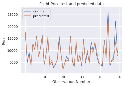
As we can observe in the above figure, model predictions and original prices are overlapping. This visual result confirms the high model score which we saw earlier.

7. Conclusion

In this article, we saw how to apply Laze Prediction library to choose the best machine learning algorithm for the task at hand.

Lazy Prediction saves time and efforts to build a machine learning model by providing model performance and training time. One can choose either based on the situation at hand.

It can also be used to build an ensemble of machine learning models. There are so many ways one can use the LazyPredict library’s functionalities.

I hope this article helped you to understand Data  Analysis, Data Preparation, and Model building approaches in a much simpler way.

Please reach out in the comment section in case of any query.

Thanks and have a good day.  🙂

The media shown in this article are not owned by Analytics Vidhya and are used at the Author’s discretion.

kajal

Hi, I am Kajal Kumari. have completed my Master’s from IIT(ISM) Dhanbad in Computer Science & Engineering. As of now, I am working as Machine Learning Engineer in Hyderabad.
hope that you have enjoyed the article. If you like it, share it with your friends also. Please feel free to comment if you have any thoughts that can improve my article writing.

If you want to read my previous blogs, you can read Previous Data Science Blog posts here. Connect with me