This article was published as a part of the Data Science Blogathon
COVID-19
COVID-19 (coronavirus disease 2019) is a disease that causes respiratory problems, fever with a temperature above 38°C, shortness of breath, and cough in humans. Even this disease can cause pneumonia to death. One of the symptoms that were considered normal before COVID-19 was a cough. Now hearing people around coughing makes others wonder whether the cough is a normal cough or the cough of someone infected with COVID-19.
What is Mel Spectrogram?
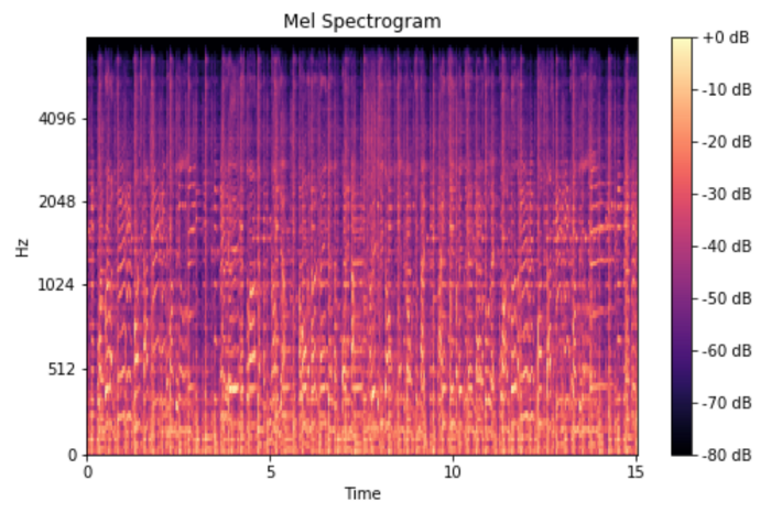
Mel spectrogram is a spectrogram that is converted to a Mel scale. Then, what is the spectrogram and The Mel Scale? A spectrogram is a visualization of the frequency spectrum of a signal, where the frequency spectrum of a signal is the frequency range that is contained by the signal. The Mel scale mimics how the human ear works, with research showing humans don’t perceive frequencies on a linear scale. Humans are better at detecting differences at lower frequencies than at higher frequencies.
Deep Learning
Deep learning is a part of artificial intelligence that makes computers learn from data. One of the methods used in deep learning is an artificial neural network which is a computational model that mimics the workings of a human neural network.
Convolutional Neural Network
A convolutional neural network is a technique in deep learning that is used to solve image processing and recognition problems. For more details on the theory of convolutional neural networks, see the blog https://www.analyticsvidhya.com/blog/category/deep-learning/.
Condition of Dataset
The voice data used can be downloaded at https://github.com/virufy/virufy-data.
The sound used data is a coughing sound recording positive for COVID-19 and negative for COVID-19. This data is in mp3 format, has a mono channel with a sample rate of 48000 Hz, and has been segmented so that it has the same time. However, can this data be used by the system to recognize the coughing sound of people infected with COVID-19? The mp3 audio format needs to be converted to wav format. Why? because what is processed in speech recognition are frequency and amplitude waves and wav is an audio format in the form of waves (waveform). Based on this, the audio needs to be preprocessed to change the format from mp3 to wav format. After this step is completed, the spectrogram mel can be obtained.
Getting an Image Mel Spectrogram from Audio
Software Audacity can be used to convert mp3 audio format to wav format. Then the audio in wav format is read using the librosa package in the python programming language. By using librosa as a package from python to analyze audio, the sample rate of 48000 Hz from the audio data obtained in the downsampling follows the default sample rate of the librosa package, so that the sample rate of the audio becomes 22050 Hz. Documentation on how to get Mel Spectrogram can be seen in the librosa documentation.
Build Model
Let’s make a system using a python programming language with Google Colab that can recognize the coughing sound of infected and non-infected people from COVID-19 from a Mel Spectrogram using a convolutional neural network.
Step 1-Import libraries
Python provides packages to make coding easier. Package used:
- Numpy for numerical analysis
- Matplotlib dan Seaborn for visualizations
- Tensorflow and Keras for deep learning
import numpy as np
import matplotlib.pyplot as plt
%matplotlib inline
from tensorflow.keras.preprocessing.image import ImageDataGenerator
import tensorflow as tf
from sklearn.metrics import confusion_matrix
import seaborn as sns
from keras.preprocessing import image
from tensorflow.keras.models import load_model
Step 2-load mel spectrogram image dataset from google drive
path_dir = './drive/My Drive/Audiodata/Cough_Covid19/mel_spectrogram/'
*Note: Google drive must be mounted to load data from google drive
Step 3-use image data generator
Image data generator is used for preprocessing image data. Rescale for resizes an image by a given scaling factor, and split the data into training and validation data where validation data is taken from 20% of the total spectrogram image data. the total dataset of the mel spectrogram image is 121, which means the validation data is 23 data.
datagen = ImageDataGenerator(
                    rescale=1./255,
                    validation_split = 0.2)
train_generator = datagen.flow_from_directory(
    path_dir,
    target_size=(150,150),
    shuffle=True,
    subset='training'
)
validation_generator = datagen.flow_from_directory(
    path_dir,
    target_size=(150,150),
    subset='validation'
)
Step 4-build a CNN model
The architecture of this CNN model:
- Conv2D layer – add 4 convolutional (16 filters, 32 filters, 64 filters, size of 3*3, and ReLU as activation function)
- Max Pooling – MaxPool2D with 2*2 layers
- Flatten layer to squeeze the layers into 1 dimension
- Dropout Layer(0.5)
- Dense, feed-forward neural network(256 nodes with ReLU as activation function
- 2 output layers with Softmax as activation function
model = tf.keras.models.Sequential([
    #first_convolution
    tf.keras.layers.Conv2D(16, (3,3), activation='relu', input_shape=(150, 150, 3)),
    tf.keras.layers.MaxPooling2D(2, 2),
    #second_convolution
    tf.keras.layers.Conv2D(32, (3,3), activation='relu'),
    tf.keras.layers.MaxPooling2D(2,2),
    #third_convolution
    tf.keras.layers.Conv2D(64, (3,3), activation='relu'),
    tf.keras.layers.MaxPooling2D(2,2),
    #fourth_convolution
    tf.keras.layers.Conv2D(64, (3,3), activation='relu'),
    tf.keras.layers.MaxPooling2D(2,2),
    tf.keras.layers.Flatten(),
    tf.keras.layers.Dropout(0.5),
    tf.keras.layers.Dense(256, activation='relu'),
    tf.keras.layers.Dense(2, activation='softmax')
])
Step 5-compile and fit model
- loss function = categorical_crossentropy
- Adam as optimizer
- batch size is 32 with 100 epochs
model.compile(loss='categorical_crossentropy', optimizer='adam', metrics=['accuracy'])
model.fit(train_generator, batch_size=32,epochs=100)
Epoch 1/100
4/4 [==============================] - 3s 481ms/step - loss: 0.6802 - accuracy: 0.5408
Epoch 2/100
4/4 [==============================] - 2s 472ms/step - loss: 0.6630 - accuracy: 0.6633
Epoch 3/100
4/4 [==============================] - 2s 720ms/step - loss: 0.6271 - accuracy: 0.6429
Epoch 4/100
4/4 [==============================] - 2s 715ms/step - loss: 0.6519 - accuracy: 0.6327
Epoch 5/100
4/4 [==============================] - 2s 504ms/step - loss: 0.5814 - accuracy: 0.6837
Epoch 6/100
4/4 [==============================] - 2s 719ms/step - loss: 0.6061 - accuracy: 0.7347
Epoch 7/100
4/4 [==============================] - 2s 506ms/step - loss: 0.5697 - accuracy: 0.7653
Epoch 8/100
4/4 [==============================] - 2s 502ms/step - loss: 0.5439 - accuracy: 0.7449
Epoch 9/100
4/4 [==============================] - 2s 500ms/step - loss: 0.5553 - accuracy: 0.7347
Epoch 10/100
4/4 [==============================] - 2s 468ms/step - loss: 0.5314 - accuracy: 0.7653
Epoch 11/100
4/4 [==============================] - 2s 723ms/step - loss: 0.5606 - accuracy: 0.7041
Epoch 12/100
4/4 [==============================] - 2s 502ms/step - loss: 0.5162 - accuracy: 0.7449
Epoch 13/100
4/4 [==============================] - 2s 498ms/step - loss: 0.5189 - accuracy: 0.7653
Epoch 14/100
4/4 [==============================] - 2s 470ms/step - loss: 0.5027 - accuracy: 0.7959
Epoch 15/100
4/4 [==============================] - 2s 713ms/step - loss: 0.5479 - accuracy: 0.7347
Epoch 16/100
4/4 [==============================] - 2s 714ms/step - loss: 0.4999 - accuracy: 0.7449
Epoch 17/100
4/4 [==============================] - 2s 469ms/step - loss: 0.5199 - accuracy: 0.7347
Epoch 18/100
4/4 [==============================] - 2s 716ms/step - loss: 0.4570 - accuracy: 0.7551
Epoch 19/100
4/4 [==============================] - 2s 474ms/step - loss: 0.4549 - accuracy: 0.7653
Epoch 20/100
4/4 [==============================] - 2s 468ms/step - loss: 0.4152 - accuracy: 0.7959
Epoch 21/100
4/4 [==============================] - 2s 509ms/step - loss: 0.4383 - accuracy: 0.7959
Epoch 22/100
4/4 [==============================] - 2s 472ms/step - loss: 0.4258 - accuracy: 0.8571
Epoch 23/100
4/4 [==============================] - 2s 465ms/step - loss: 0.3988 - accuracy: 0.8469
Epoch 24/100
4/4 [==============================] - 2s 705ms/step - loss: 0.4435 - accuracy: 0.8163
Epoch 25/100
4/4 [==============================] - 2s 478ms/step - loss: 0.3931 - accuracy: 0.7959
Epoch 26/100
4/4 [==============================] - 2s 473ms/step - loss: 0.3964 - accuracy: 0.8469
Epoch 27/100
4/4 [==============================] - 2s 721ms/step - loss: 0.4285 - accuracy: 0.7551
Epoch 28/100
4/4 [==============================] - 2s 504ms/step - loss: 0.3571 - accuracy: 0.8163
Epoch 29/100
4/4 [==============================] - 2s 476ms/step - loss: 0.3053 - accuracy: 0.8878
Epoch 30/100
4/4 [==============================] - 2s 505ms/step - loss: 0.4531 - accuracy: 0.7245
Epoch 31/100
4/4 [==============================] - 2s 461ms/step - loss: 0.4956 - accuracy: 0.7653
Epoch 32/100
4/4 [==============================] - 2s 712ms/step - loss: 0.3593 - accuracy: 0.8367
Epoch 33/100
4/4 [==============================] - 2s 499ms/step - loss: 0.3291 - accuracy: 0.8673
Epoch 34/100
4/4 [==============================] - 2s 471ms/step - loss: 0.2828 - accuracy: 0.8571
Epoch 35/100
4/4 [==============================] - 2s 719ms/step - loss: 0.2740 - accuracy: 0.8776
Epoch 36/100
4/4 [==============================] - 2s 511ms/step - loss: 0.3409 - accuracy: 0.8776
Epoch 37/100
4/4 [==============================] - 2s 463ms/step - loss: 0.2144 - accuracy: 0.9082
Epoch 38/100
4/4 [==============================] - 2s 474ms/step - loss: 0.1550 - accuracy: 0.9490
Epoch 39/100
4/4 [==============================] - 2s 708ms/step - loss: 0.2104 - accuracy: 0.9184
Epoch 40/100
4/4 [==============================] - 2s 483ms/step - loss: 0.2203 - accuracy: 0.9184
Epoch 41/100
4/4 [==============================] - 2s 715ms/step - loss: 0.2048 - accuracy: 0.9184
Epoch 42/100
4/4 [==============================] - 2s 472ms/step - loss: 0.1701 - accuracy: 0.8980
Epoch 43/100
4/4 [==============================] - 2s 473ms/step - loss: 0.1755 - accuracy: 0.9490
Epoch 44/100
4/4 [==============================] - 2s 468ms/step - loss: 0.1723 - accuracy: 0.9388
Epoch 45/100
4/4 [==============================] - 2s 710ms/step - loss: 0.1240 - accuracy: 0.9796
Epoch 46/100
4/4 [==============================] - 2s 710ms/step - loss: 0.1356 - accuracy: 0.9388
Epoch 47/100
4/4 [==============================] - 2s 461ms/step - loss: 0.1046 - accuracy: 0.9592
Epoch 48/100
4/4 [==============================] - 2s 708ms/step - loss: 0.2454 - accuracy: 0.8878
Epoch 49/100
4/4 [==============================] - 2s 473ms/step - loss: 0.1540 - accuracy: 0.9286
Epoch 50/100
4/4 [==============================] - 2s 705ms/step - loss: 0.1769 - accuracy: 0.9592
Epoch 51/100
4/4 [==============================] - 2s 510ms/step - loss: 0.1795 - accuracy: 0.9184
Epoch 52/100
4/4 [==============================] - 2s 497ms/step - loss: 0.1267 - accuracy: 0.9592
Epoch 53/100
4/4 [==============================] - 2s 472ms/step - loss: 0.0952 - accuracy: 0.9694
Epoch 54/100
4/4 [==============================] - 2s 467ms/step - loss: 0.0974 - accuracy: 0.9592
Epoch 55/100
4/4 [==============================] - 2s 473ms/step - loss: 0.0629 - accuracy: 0.9898
Epoch 56/100
4/4 [==============================] - 2s 468ms/step - loss: 0.0995 - accuracy: 0.9592
Epoch 57/100
4/4 [==============================] - 2s 472ms/step - loss: 0.0487 - accuracy: 0.9694
Epoch 58/100
4/4 [==============================] - 2s 718ms/step - loss: 0.0348 - accuracy: 0.9898
Epoch 59/100
4/4 [==============================] - 2s 504ms/step - loss: 0.0419 - accuracy: 0.9898
Epoch 60/100
4/4 [==============================] - 2s 507ms/step - loss: 0.0490 - accuracy: 0.9796
Epoch 61/100
4/4 [==============================] - 2s 506ms/step - loss: 0.0608 - accuracy: 0.9796
Epoch 62/100
4/4 [==============================] - 2s 507ms/step - loss: 0.0877 - accuracy: 0.9490
Epoch 63/100
4/4 [==============================] - 2s 476ms/step - loss: 0.1254 - accuracy: 0.9490
Epoch 64/100
4/4 [==============================] - 2s 705ms/step - loss: 0.0537 - accuracy: 0.9898
Epoch 65/100
4/4 [==============================] - 2s 711ms/step - loss: 0.1157 - accuracy: 0.9592
Epoch 66/100
4/4 [==============================] - 2s 512ms/step - loss: 0.0403 - accuracy: 0.9898
Epoch 67/100
4/4 [==============================] - 2s 506ms/step - loss: 0.0734 - accuracy: 0.9796
Epoch 68/100
4/4 [==============================] - 2s 727ms/step - loss: 0.1231 - accuracy: 0.9592
Epoch 69/100
4/4 [==============================] - 2s 502ms/step - loss: 0.0822 - accuracy: 0.9694
Epoch 70/100
4/4 [==============================] - 2s 470ms/step - loss: 0.0897 - accuracy: 0.9694
Epoch 71/100
4/4 [==============================] - 2s 498ms/step - loss: 0.0543 - accuracy: 0.9592
Epoch 72/100
4/4 [==============================] - 2s 711ms/step - loss: 0.0235 - accuracy: 0.9898
Epoch 73/100
4/4 [==============================] - 2s 474ms/step - loss: 0.0425 - accuracy: 0.9898
Epoch 74/100
4/4 [==============================] - 2s 498ms/step - loss: 0.0373 - accuracy: 0.9898
Epoch 75/100
4/4 [==============================] - 2s 471ms/step - loss: 0.0220 - accuracy: 0.9898
Epoch 76/100
4/4 [==============================] - 2s 710ms/step - loss: 0.0274 - accuracy: 0.9898
Epoch 77/100
4/4 [==============================] - 2s 708ms/step - loss: 0.0256 - accuracy: 1.0000
Epoch 78/100
4/4 [==============================] - 2s 707ms/step - loss: 0.0137 - accuracy: 1.0000
Epoch 79/100
4/4 [==============================] - 2s 470ms/step - loss: 0.0123 - accuracy: 1.0000
Epoch 80/100
4/4 [==============================] - 2s 516ms/step - loss: 0.0278 - accuracy: 0.9796
Epoch 81/100
4/4 [==============================] - 2s 478ms/step - loss: 0.0311 - accuracy: 0.9796
Epoch 82/100
4/4 [==============================] - 2s 477ms/step - loss: 0.0318 - accuracy: 0.9796
Epoch 83/100
4/4 [==============================] - 2s 472ms/step - loss: 0.0184 - accuracy: 0.9898
Epoch 84/100
4/4 [==============================] - 2s 477ms/step - loss: 0.0191 - accuracy: 1.0000
Epoch 85/100
4/4 [==============================] - 2s 480ms/step - loss: 0.0146 - accuracy: 1.0000
Epoch 86/100
4/4 [==============================] - 2s 726ms/step - loss: 0.0047 - accuracy: 1.0000
Epoch 87/100
4/4 [==============================] - 2s 508ms/step - loss: 0.0072 - accuracy: 1.0000
Epoch 88/100
4/4 [==============================] - 2s 475ms/step - loss: 0.0049 - accuracy: 1.0000
Epoch 89/100
4/4 [==============================] - 2s 470ms/step - loss: 0.0169 - accuracy: 0.9898
Epoch 90/100
4/4 [==============================] - 2s 730ms/step - loss: 0.0048 - accuracy: 1.0000
Epoch 91/100
4/4 [==============================] - 2s 479ms/step - loss: 0.0117 - accuracy: 0.9898
Epoch 92/100
4/4 [==============================] - 2s 521ms/step - loss: 0.0018 - accuracy: 1.0000
Epoch 93/100
4/4 [==============================] - 2s 714ms/step - loss: 0.0066 - accuracy: 1.0000
Epoch 94/100
4/4 [==============================] - 2s 509ms/step - loss: 0.0198 - accuracy: 0.9898
Epoch 95/100
4/4 [==============================] - 2s 513ms/step - loss: 0.0193 - accuracy: 0.9898
Epoch 96/100
4/4 [==============================] - 2s 479ms/step - loss: 0.0048 - accuracy: 1.0000
Epoch 97/100
4/4 [==============================] - 2s 711ms/step - loss: 0.0064 - accuracy: 1.0000
Epoch 98/100
4/4 [==============================] - 2s 467ms/step - loss: 0.0283 - accuracy: 0.9796
Epoch 99/100
4/4 [==============================] - 2s 470ms/step - loss: 0.0043 - accuracy: 1.0000
Epoch 100/100
4/4 [==============================] - 2s 470ms/step - loss: 0.0113 - accuracy: 0.9898
Model training accuracy is 0.9898 (98.98%) and loss is 0.0113.
Step 6-evaluate model and predict
The last part is to evaluate the data using data validation data (validation generator).
accuracy = model.evaluate(validation_generator)
print('n', 'Test_Accuracy:-', accuracy[1])
pred = model.predict(validation_generator)
y_pred = np.argmax(pred, axis=1)
y_true = np.argmax(pred, axis=1)
print('confusion matrix')
print(confusion_matrix(y_true, y_pred))
    #confusion matrix
f, ax = plt.subplots(figsize=(8,5))
sns.heatmap(confusion_matrix(y_true, y_pred), annot=True, fmt=".0f", ax=ax)
plt.xlabel("y_pred")
plt.ylabel("y_true")
plt.show()
Result
The accuracy of the model evaluate to 0.9565 (95.65%)
- 23 test data
- 0 indicates negative infected COVID-19
- 1 indicates positive infected COVID-19
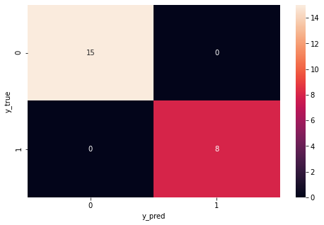
Confusion Matrix of Testing Data
Based on the confusion matrix, the system has no errors in predicting data, which means this model has a fairly good system performance in recognizing coughs that are infected with COVID-19 and not infected with COVID-19 through Mel Spectrogram images.
However, this model still needs a lot of development.
About The Author
Abdiel Willyar Goni
Currently pursuing my bachelor’s degree in mathematics. I am interested in machine learning, computer vision, and signal processing. Feel free to connect with me on LinkedIn
Thank you.
The media shown in this article are not owned by Analytics Vidhya and are used at the Author’s discretion.


Very creative and cool experiment. Kudos!