Make your Images Clearer and Crisper – Denoise Images with Autoencoders
This article was published as a part of the Data Science Blogathon
Introduction
“Tools can be the same for everyone, but how a wielder use it makes the difference”
We often think that we should be aware of all the services or tools that are out there in the market to fulfill a required task. Well, I agree with this mentality so much so you can keep exploring and keep experimenting with different combinations of tools to produce useful inferences. But this doesn’t mean that I don’t favor the mentality of thinking creatively with what you already have. Many of the times, we all have a certain range of knowledge regarding any domains and promoters that can make the work easy and simple and at the same time no 2 people can know exactly the same amount and type of knowledge. This would mean that we all are unaware of various possibilities that collectively other people might know.
Today, I will try to focus on the idea of thinking creatively with what you already know.
This article talks about a very popular technique or architecture in deep learning to handle various unsupervised learning problems: AutoEncoders.
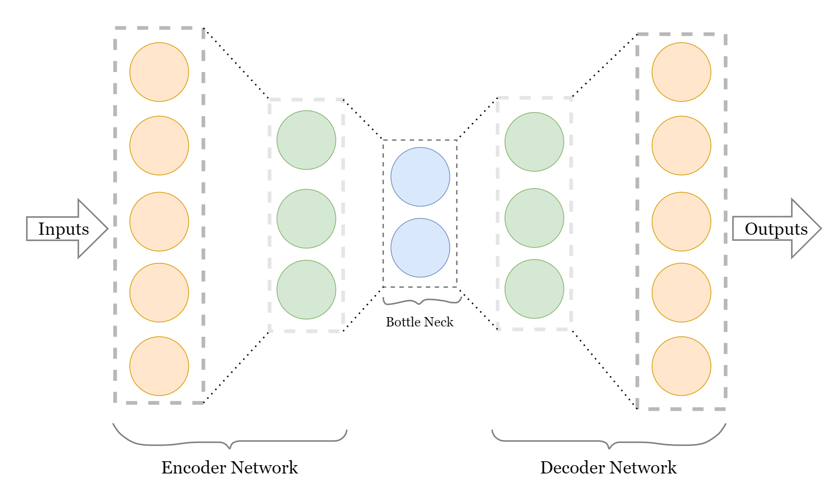
AutoEncoders is a name given to a specific type of neural network architecture that comprises 2 networks connected to each other by a bottleneck layer (latent dimension layer). These 2 networks are opposite in terms of their functionality and what they provide with their execution. The first network is called an Encoder, which takes the input examples and generates numerical values to represent that data in smaller dimensions (latent dimension). The encoded data is targeted to be responsible for understanding the raw input in a lower number of values (saving the nature and features of the raw input as much as possible). This output that you get as a smaller dimension encoded representation of input data is what we call a bottleneck layer(latent dimension layer).
The second network in the architecture is connected just after the bottleneck layer, making the network work in continuation as those latent dimensions are now the input to the second network, also known as Decoder.
Here is how a basic Autoencoder network looks like:
Let us look at the code to teach a neural network, how to generate images from the fashion MNIST dataset. Check more information about the dataset on the attached link and for your brief understanding, just know that this dataset contains greyscale images of size (28,28) which have 10 classes based on fashion clothing objects.
Importing necessary libraries/modules:
import tensorflow as tf
import numpy as np
import matplotlib.pyplot as plt
import pandas as pd
from tensorflow.keras.datasets import fashion_mnist
from tensorflow.keras import layers, losses
from tensorflow.keras.models import Model
1. Retrieve the data
Once, we retrieve the data from tensorflow.keras.datasets, we need to rescale the values of pixel range from (0-255) to (0,1), and for such we will divide all the pixel values with 255.0 to normalize them. NOTE: As autoencoders are capable of unsupervised learning (without Labels) and this is what we wish to achieve through this article, we will ignore labels from the training and testing dataset for fashionMNIST.
(x_train, _), (x_test, _) = fashion_mnist.load_data()
x_train = x_train.astype('float32')/255.
x_test = x_test.astype('float32')/255.
print(x_train.shape)
print(x_test.shape)
As you can see, after running this code, we have 60,000 thousand training images and 10,000 testing images.
2. Adding the Noise
The raw dataset doesn’t contain any noise in the images but for our task, we can only learn to denoise the images that have noise already in them. So for our case, let’s add some noise in our data.
Here we are working with greyscale images, that have only 1 channel but that channel is not mentioned as an additional dimension in the dataset, so for the purpose of adding noise, we need to add a dimension of value ‘1’, which corresponds to the greyscale channel for each image in the training and testing set.
x_train = x_train[..., tf.newaxis]
x_test = x_test[..., tf.newaxis]
print(x_train.shape)
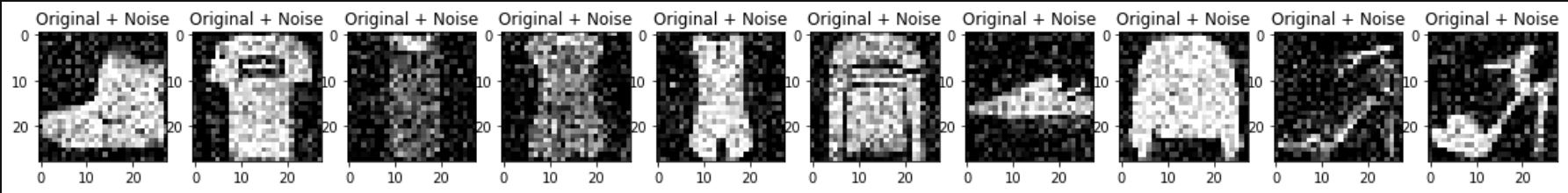
## Adding Noise, with Noise intensity handled by noise_factor
noise_factor = 0.2
x_train_noisy = x_train + noise_factor*tf.random.normal(shape=x_train.shape)
x_test_noisy = x_test + noise_factor * tf.random.normal(shape=x_test.shape)
x_train_noisy = tf.clip_by_value(x_train_noisy, clip_value_min = 0., clip_value_max = 1.)
x_test_noisy = tf.clip_by_value(x_test_noisy, clip_value_min = 0., clip_value_max = 1.)
Let’s visualize these noisy images:
n = 10
plt.figure(figsize=(20,2))
for i in range(n):
    plt.subplot(1, n, i+1)
    plt.imshow(tf.squeeze(x_train_noisy[i]))
    plt.title('Original + Noise')
    plt.gray()
plt.show()
3. Create a Convolutional Autoencoder network
we create this convolutional autoencoder network to learn the meaningful representation of these images their significantly important features. Through this understanding, we will be able to generate a denoised version of this dataset from the latent dimensional values of these images.
class Conv_AutoEncoder(Model):
    def __init__(self):
        super(Conv_AutoEncoder, self).__init__()
        self.encoder = tf.keras.Sequential([
            layers.Input(shape=(28,28,1)),
            layers.Conv2D(16, (3,3), activation='relu', padding='same', strides=2),
            layers.Conv2D(8, (3,3), activation='relu', padding='same', strides=2)
        ])
        self.decoder = tf.keras.Sequential([
            layers.Conv2DTranspose(8, kernel_size=3, strides = 2, activation='relu', padding='same'),
            layers.Conv2DTranspose(16, kernel_size=3, strides=2, activation='relu', padding='same',),
            layers.Conv2D(1, kernel_size=(3,3), activation='sigmoid', padding='same')
        ])
    def call(self,x):
        encoded = self.encoder(x)
        decoded = self.decoder(encoded)
        return decoded
conv_autoencoder = Conv_AutoEncoder()
conv_autoencoder.compile(loss=losses.MeanSquaredError(), optimizer = 'adam')
We have created this network using TensorFlow’s Subclassing API. We inherited the Model class in our Conv_AutoEncoder class and defined the network as individual methods to this class (self.encoder and self.decoder).
Encoder: We have chosen an extremely basic model architecture for the demonstration purpose, which consists of an Input Layer, 2 Convolutional 2D layers.
Decoder: For upsampling the images to their original size through transpose convolutions, we are using 2 Convolutional2D Transpose layers and 1 mainstream convolutional 2D layer to get the channel dimension as 1 (same as for grayscale images).
Small to-do task for you: use conv_autoencoder.encoder.summary() and conv_autoencoder.decoder.summary() to observe a more detailed architecture of these networks.
4. Training the Model and Testing it
As discussed above already, we don’t have labels for these images, but what we do have is original images and noisy images, we can train our model to understand the representation of original images from latent space created by noisy images. This will give us a trained decoder network to remove the noise from the noisy image’s latent representations and get clearer images.
TRAINING:
conv_autoencoder.fit(x_train_noisy, x_train, epochs=10, validation_data = (x_test_noisy, x_test))
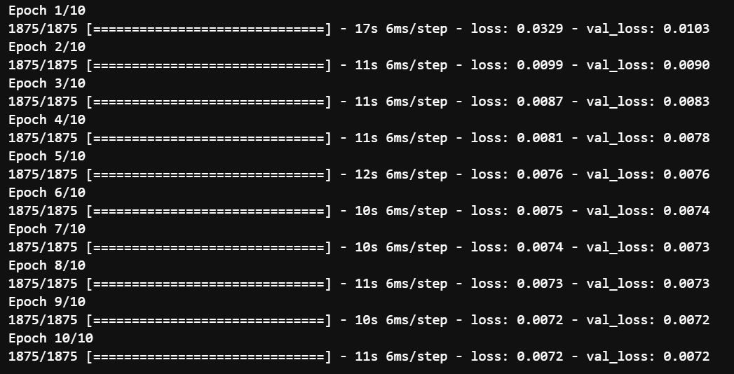
Training loss and validation loss, both seem to be almost exact which means there is no overfitting and also there is no significant decrease in both the losses for the last 4 epochs, which says that it has reached the almost optimal representation between the images.
TESTING:
conv_encoded_images = conv_autoencoder.encoder(x_test_noisy).numpy()
conv_decoded_images = conv_autoencoder.decoder(conv_encoded_images).numpy()
Visualizing the Effect of Denoising:
n = 10
plt.figure(figsize=(20, 4))
for i in range(n):
    # display original
    ax = plt.subplot(2, n, i + 1)
    plt.imshow(x_test_noisy[i])
    plt.title("original")
    plt.gray()
    ax.get_xaxis().set_visible(False)
    ax.get_yaxis().set_visible(False)
    # display reconstruction
    ax = plt.subplot(2, n, i + 1 + n)
    plt.imshow(conv_decoded_images[i])
    plt.title("reconstructed")
    plt.gray()
    ax.get_xaxis().set_visible(False)
    ax.get_yaxis().set_visible(False)
plt.show()
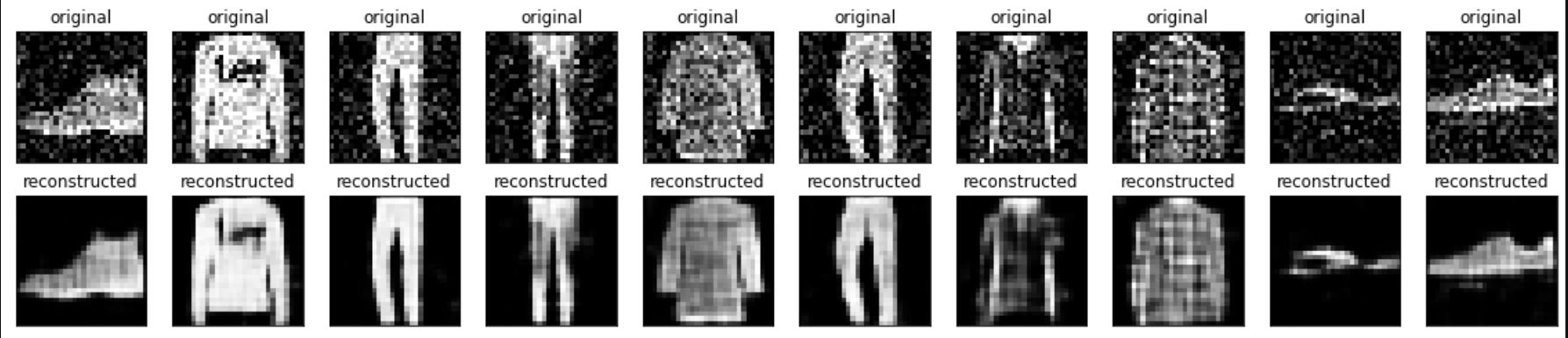
Well, that was it for this article, I hope you understood the basic functionality of autoencoders and how they can be used for reducing the noise in images.
Gargeya Sharma
B.Tech 3rd Year Student
Specialized in Deep Learning and Data Science
For getting more info check out my Github Homepage
The media shown in this article are not owned by Analytics Vidhya and are used at the Author’s discretion.


