This article was published as a part of the Data Science Blogathon
Introduction
We have an input layer, a hidden layer, and an output layer. The input layer takes the input, activations functions are applied to the hidden layer, and finally, we receive the output.
In a deep neural network where multiple hidden layers are present. Each hidden layer is known by its weights and biases.
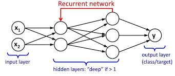
The weights and biases of these hidden layers are different. Hence each of these layers behaves differently/independently and so that we can’t combine them together. We should have the same weights and biases for these hidden layers to bind these hidden layers together.
Now we can combine these layers together because the weights and bias of all the hidden layers are the same now. All these hidden layers can be bound together in one single recurrent layer.
There are three types of Deep Neural Networks:
1. Artificial Neural Network
2. Convolutional Neural Network
3. Recurrent Neural Network
In this article, we will be focusing on Recurrent Neural Networks.
What are RNNs?
– A series of feed-forward neural networks in which the hidden nodes are connected in series.
– RNN has multiple series predictions, unlike CNN.
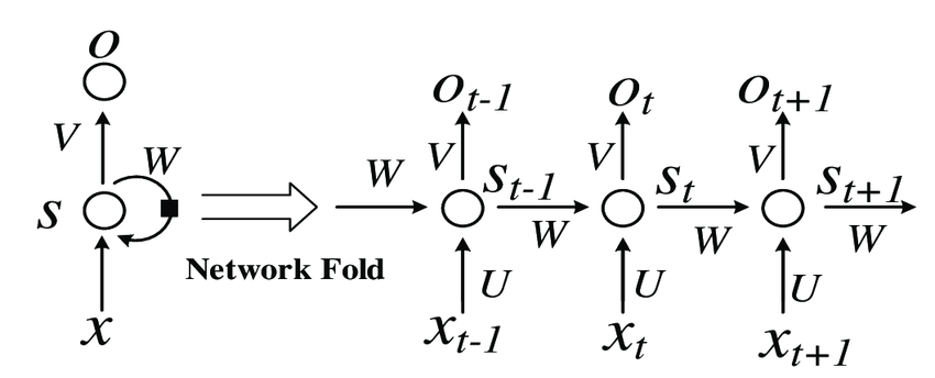
Image source: https://www.researchgate.net/publication/329330308/figure/fig1/AS:698826503495682@1543624630550/Basic-recurrent-neural-network-RNN-structure.png
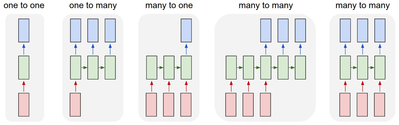
Types of RNNs
1. One to One: This is also called Vanilla Neural Network. It is used in such machine learning problems where it has a single input and single output
2. One to Many: It has a single input and multiple outputs. An example is Music Generation
3. Many to One: RNN takes a sequence of inputs and produces a single output. The examples are Sentiment classification, prediction of the next word.
4. Many to Many: RNN takes a sequence of inputs and produces a sequence of outputs. For example, Language Translation.
Improvements to RNN
– RNNs have a problem called vanishing gradient descent
– Hence there are two improvements over it
1.Gated Recurrent Unit (GRU)
2.Long Short Term Memory (LSTM))
– Among these more popular is LSTM more often used in time series
forecasting also.
Vanishing Gradient Problem
Before we build our first RNN, we need to understand the vanishing gradient problem. Let’s take a quick look at Vanishing Gradient Problem.
What is the Vanishing Gradient Problem?
The Vanishing Gradient Problem was discovered by Sepp Hochreiter, who is a German computer scientist who also had a role in the development of Recurrent Neural Networks in deep learning.
As its name says, the vanishing gradient problem is related to deep learning gradient descent algorithms. The gradient descent algorithm is then combined with a backpropagation algorithm to update the weights throughout the Neural Network. Recurrent neural network behaves a little differently due to the hidden layer of one observation is used to train the hidden layer of the next observation.
This vanishing gradient problem occurs when the backpropagation algorithm moves back through all the neurons of the neural network to update their weights.
Initialization of weights is one of the techniques that can be used to solve the Vanishing Gradient Problem. That is creating an initial value for weights in a neural network to prevent the backpropagation algorithm from assigning weights that are small.
Applications(Some of) of RNN
– Speech Recognition: Anyone speaking with a particular language, gets translated into different languages. And also voice is recognized by the machine.
– Language Translation: Using RNN, Text mining and Sentiment analysis can be carried out for Natural Language Processing (NLP).
– Image Recognition and its characterization: RNNs are used to capture an image by analyzing the present activities.
– Time Series Forecasting: Any time series forecasting problem, such as predicting the prices of stocks in a particular month/year, can be solved using an RNN.
Implementation Of RNN
Let us look at how to implement Time Series Forecasting using LSTM(Long Short Term Memory).
Now we will import some basic libraries to perform data frame functions.
Here I have used a dataset of Google Stock Price. You can download the dataset using this link. So there are two files in the given dataset as google_stock_price_train.csv and google_stock_price_test.csv. So first here we are going to take the training file.
import numpy as np
import matplotlib.pyplot as plt
import pandas as pd
dataset_train = pd.read_csv('Google_Stock_Price_Train.csv')
print(dataset_train.shape)
training_set = dataset_train.iloc[:, 1:2].values
Next, we have to perform normalization of data using scaling. Our data will be scaled into a specific format. So we need the MinMaxScaler library as well.
from sklearn.preprocessing import MinMaxScaler
sc = MinMaxScaler(feature_range = (0, 1))
training_set_scaled = sc.fit_transform(training_set)
Now, we create a data structure with 60 timesteps and one output as an Array of x_train and y_train.
X_train = []
y_train = []
for i in range(60, 1258):
    X_train.append(training_set_scaled[i-60:i, 0])
    y_train.append(training_set_scaled[i, 0])
X_train, y_train = np.array(X_train), np.array(y_train)
Here we have done reshaping of x_train data.
X_train = np.reshape(X_train, (X_train.shape[0], X_train.shape[1], 1))
Now, the following libraries are required for building the RNN model and perform its operations. We have imported the Keras library and its packages.
from keras.models import Sequential
from keras.layers import Dense
from keras.layers import LSTM
from keras.layers import Dropout
Let’s initialize our RNN.
regressor = Sequential()
Now, add the first layer of LSTM and some Dropout regularisation
regressor.add(LSTM(units = 50, return_sequences = True, input_shape = (X_train.shape[1], 1)))
regressor.add(Dropout(0.2))
Now, add the second layer of LSTM and some Dropout regularisation
regressor.add(LSTM(units = 50, return_sequences = True))
regressor.add(Dropout(0.2))
Now, add the third layer of LSTM and some Dropout regularisation
regressor.add(LSTM(units = 50, return_sequences = True))
regressor.add(Dropout(0.2))
Now, add the fourth layer of LSTM and some Dropout regularisation
regressor.add(LSTM(units = 50))
regressor.add(Dropout(0.2))
Let’s add an output layer.
regressor.add(Dense(units = 1))
Next, we will compile our RNN model here.
regressor.compile(optimizer = 'adam', loss = 'mean_squared_error')
We are using a training dataset to fit the RNN model.
regressor.fit(X_train, y_train, epochs = 100, batch_size = 32)
Epoch 1/100
38/38 [==============================] - 4s 100ms/step - loss: 0.0419 0s - loss:
Epoch 2/100
38/38 [==============================] - 4s 104ms/step - loss: 0.0058
Epoch 3/100
38/38 [==============================] - 4s 99ms/step - loss: 0.0060
Epoch 4/100
38/38 [==============================] - 4s 98ms/step - loss: 0.0051
Epoch 5/100
38/38 [==============================] - 4s 100ms/step - loss: 0.0050
Epoch 6/100
38/38 [==============================] - 4s 99ms/step - loss: 0.0045
Epoch 7/100
38/38 [==============================] - 4s 101ms/step - loss: 0.0047
Epoch 8/100
38/38 [==============================] - 4s 100ms/step - loss: 0.0046
Epoch 9/100
38/38 [==============================] - 4s 101ms/step - loss: 0.0044
Epoch 10/100
38/38 [==============================] - 4s 103ms/step - loss: 0.0046
Epoch 11/100
38/38 [==============================] - 4s 103ms/step - loss: 0.0043
Epoch 12/100
38/38 [==============================] - 4s 101ms/step - loss: 0.0041
Epoch 13/100
38/38 [==============================] - 4s 100ms/step - loss: 0.0047
Epoch 14/100
38/38 [==============================] - 4s 100ms/step - loss: 0.0035
Epoch 15/100
38/38 [==============================] - 4s 100ms/step - loss: 0.0039
Epoch 16/100
38/38 [==============================] - 4s 100ms/step - loss: 0.0038
Epoch 17/100
38/38 [==============================] - 4s 100ms/step - loss: 0.0035
Epoch 18/100
38/38 [==============================] - 4s 100ms/step - loss: 0.0035
Epoch 19/100
38/38 [==============================] - 4s 100ms/step - loss: 0.0034
Epoch 20/100
38/38 [==============================] - 4s 100ms/step - loss: 0.0036
Epoch 21/100
38/38 [==============================] - 4s 102ms/step - loss: 0.0038
Epoch 22/100
38/38 [==============================] - 4s 100ms/step - loss: 0.0034
Epoch 23/100
38/38 [==============================] - 4s 101ms/step - loss: 0.0033
Epoch 24/100
38/38 [==============================] - 4s 101ms/step - loss: 0.0036
Epoch 25/100
38/38 [==============================] - 4s 102ms/step - loss: 0.0035
Epoch 26/100
38/38 [==============================] - 4s 102ms/step - loss: 0.0036
Epoch 27/100
38/38 [==============================] - 4s 102ms/step - loss: 0.0031
Epoch 28/100
38/38 [==============================] - 4s 106ms/step - loss: 0.0032
Epoch 29/100
38/38 [==============================] - 4s 103ms/step - loss: 0.0030
Epoch 30/100
38/38 [==============================] - 4s 102ms/step - loss: 0.0030
Epoch 31/100
38/38 [==============================] - 4s 102ms/step - loss: 0.0031
Epoch 32/100
38/38 [==============================] - 4s 101ms/step - loss: 0.0030 0s - lo
Epoch 33/100
38/38 [==============================] - 4s 103ms/step - loss: 0.0028
Epoch 34/100
38/38 [==============================] - 4s 102ms/step - loss: 0.0030
Epoch 35/100
38/38 [==============================] - 4s 101ms/step - loss: 0.0025
Epoch 36/100
38/38 [==============================] - 4s 101ms/step - loss: 0.0028
Epoch 37/100
38/38 [==============================] - 4s 101ms/step - loss: 0.0032
Epoch 38/100
38/38 [==============================] - 4s 102ms/step - loss: 0.0028
Epoch 39/100
38/38 [==============================] - 4s 102ms/step - loss: 0.0031
Epoch 40/100
38/38 [==============================] - 4s 102ms/step - loss: 0.0026
Epoch 41/100
38/38 [==============================] - 4s 102ms/step - loss: 0.0026
Epoch 42/100
38/38 [==============================] - 4s 106ms/step - loss: 0.0027
Epoch 43/100
38/38 [==============================] - 4s 105ms/step - loss: 0.0027
Epoch 44/100
38/38 [==============================] - 4s 104ms/step - loss: 0.0023
Epoch 45/100
38/38 [==============================] - 4s 106ms/step - loss: 0.0023
Epoch 46/100
38/38 [==============================] - 4s 103ms/step - loss: 0.0024
Epoch 47/100
38/38 [==============================] - 4s 103ms/step - loss: 0.0024 0s - loss: 0.002
Epoch 48/100
38/38 [==============================] - 4s 103ms/step - loss: 0.0025
Epoch 49/100
38/38 [==============================] - 4s 103ms/step - loss: 0.0025 0s - lo
Epoch 50/100
38/38 [==============================] - 4s 103ms/step - loss: 0.0023
Epoch 51/100
38/38 [==============================] - 4s 102ms/step - loss: 0.0023
Epoch 52/100
38/38 [==============================] - 4s 102ms/step - loss: 0.0024
Epoch 53/100
38/38 [==============================] - 4s 102ms/step - loss: 0.0022
Epoch 54/100
38/38 [==============================] - 4s 103ms/step - loss: 0.0023
Epoch 55/100
38/38 [==============================] - 4s 103ms/step - loss: 0.0022
Epoch 56/100
38/38 [==============================] - 4s 102ms/step - loss: 0.0025 0s - loss
Epoch 57/100
38/38 [==============================] - 4s 103ms/step - loss: 0.0023
Epoch 58/100
38/38 [==============================] - 4s 102ms/step - loss: 0.0022
Epoch 59/100
38/38 [==============================] - 4s 103ms/step - loss: 0.0022
Epoch 60/100
38/38 [==============================] - 4s 103ms/step - loss: 0.0021
Epoch 61/100
38/38 [==============================] - 4s 109ms/step - loss: 0.0021
Epoch 62/100
38/38 [==============================] - 4s 105ms/step - loss: 0.0020
Epoch 63/100
38/38 [==============================] - 4s 102ms/step - loss: 0.0020
Epoch 64/100
38/38 [==============================] - 4s 102ms/step - loss: 0.0022 0s - loss: 0.0 - ETA: 0s - loss: 0.002
Epoch 65/100
38/38 [==============================] - 4s 103ms/step - loss: 0.0024
Epoch 66/100
38/38 [==============================] - 4s 103ms/step - loss: 0.0021
Epoch 67/100
38/38 [==============================] - 4s 102ms/step - loss: 0.0020
Epoch 68/100
38/38 [==============================] - 4s 103ms/step - loss: 0.0019
Epoch 69/100
38/38 [==============================] - 4s 102ms/step - loss: 0.0020
Epoch 70/100
38/38 [==============================] - 4s 106ms/step - loss: 0.0022
Epoch 71/100
38/38 [==============================] - 4s 103ms/step - loss: 0.0020
Epoch 72/100
38/38 [==============================] - 4s 102ms/step - loss: 0.0018
Epoch 73/100
38/38 [==============================] - 4s 103ms/step - loss: 0.0020
Epoch 74/100
38/38 [==============================] - 4s 102ms/step - loss: 0.0016
Epoch 75/100
38/38 [==============================] - 4s 104ms/step - loss: 0.0018
Epoch 76/100
38/38 [==============================] - 4s 103ms/step - loss: 0.0018
Epoch 77/100
38/38 [==============================] - 4s 106ms/step - loss: 0.0019
Epoch 78/100
38/38 [==============================] - 4s 105ms/step - loss: 0.0017
Epoch 79/100
38/38 [==============================] - 4s 104ms/step - loss: 0.0019
Epoch 80/100
38/38 [==============================] - 4s 111ms/step - loss: 0.0018
Epoch 81/100
38/38 [==============================] - 5s 123ms/step - loss: 0.0017
Epoch 82/100
38/38 [==============================] - 4s 104ms/step - loss: 0.0017
Epoch 83/100
38/38 [==============================] - 4s 102ms/step - loss: 0.0017
Epoch 84/100
38/38 [==============================] - 4s 102ms/step - loss: 0.0015
Epoch 85/100
38/38 [==============================] - 4s 104ms/step - loss: 0.0015
Epoch 86/100
38/38 [==============================] - 4s 102ms/step - loss: 0.0015 0s - los
Epoch 87/100
38/38 [==============================] - 4s 101ms/step - loss: 0.0018
Epoch 88/100
38/38 [==============================] - 4s 102ms/step - loss: 0.0015
Epoch 89/100
38/38 [==============================] - 4s 102ms/step - loss: 0.0015 1s
Epoch 90/100
38/38 [==============================] - 4s 101ms/step - loss: 0.0017
Epoch 91/100
38/38 [==============================] - 4s 101ms/step - loss: 0.0017
Epoch 92/100
38/38 [==============================] - 4s 101ms/step - loss: 0.0017
Epoch 93/100
38/38 [==============================] - 4s 103ms/step - loss: 0.0014
Epoch 94/100
38/38 [==============================] - 4s 104ms/step - loss: 0.0017
Epoch 95/100
38/38 [==============================] - 4s 102ms/step - loss: 0.0016
Epoch 96/100
38/38 [==============================] - 4s 102ms/step - loss: 0.0013
Epoch 97/100
38/38 [==============================] - 4s 102ms/step - loss: 0.0014
Epoch 98/100
38/38 [==============================] - 4s 101ms/step - loss: 0.0015
Epoch 99/100
38/38 [==============================] - 4s 102ms/step - loss: 0.0014
Epoch 100/100
38/38 [==============================] - 4s 101ms/step - loss: 0.0014
Now our next part is to predict stock prices and visualize their results. Here we have used the real stock price of 2017 with data of google_stock_price.csv.
dataset_test = pd.read_csv('Google_Stock_Price_Test.csv')
real_stock_price = dataset_test.iloc[:, 1:2].values
Getting the predicted stock price of 2017
dataset_total = pd.concat((dataset_train['Open'], dataset_test['Open']), axis = 0)
inputs = dataset_total[len(dataset_total) - len(dataset_test) - 60:].values
inputs = inputs.reshape(-1,1)
inputs = sc.transform(inputs)
X_test = []
for i in range(60, 80):
    X_test.append(inputs[i-60:i, 0])
X_test = np.array(X_test)
X_test = np.reshape(X_test, (X_test.shape[0], X_test.shape[1], 1))
predicted_stock_price = regressor.predict(X_test)
predicted_stock_price = sc.inverse_transform(predicted_stock_price)
The final step is to visualize our data results using the matplotlib library.
plt.plot(real_stock_price, color = 'red', label = 'Real Google Stock Price')
plt.plot(predicted_stock_price, color = 'blue', label = 'Predicted Google Stock Price')
plt.title('Google Stock Price Prediction')
plt.xlabel('Time')
plt.ylabel('Google Stock Price')
plt.legend()
plt.show()
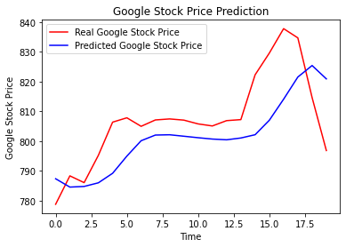
Shown image is a graph plotted by the above code.
Conclusion
Finally… We have successfully built our Basic Time Series Analysis model using Recurrent Neural Network. I hope you liked my article. Do share with your friends and colleagues. Thank You!
The media shown in this article are not owned by Analytics Vidhya and are used at the Author’s discretion.
I am Software Engineer, data enthusiast , passionate about data and its potential to drive insights, solve problems and also seeking to learn more about machine learning, artificial intelligence fields.


why you are passing the 50 units, what does it mean.. regressor.add(LSTM(units = 50, return_sequences = True, input_shape = (X_train.shape[1], 1)))
Hi Mrs. Amruta, I hope your are doing well. I am very exciting for this knowledge shared. Very thankful to you.