This article was published as a part of the Data Science Blogathon
What is transfer learning?
We’re always told that “Practice makes a man perfect” and we’re made to practice tons of problems in different domains to prepare us for the doom day i.e our final exam. The more variety of problems we solve, the better we get at transferring that knowledge to solve a new problem. What if there’s a way to apply the same technique to solve classification, regression, or clustering problems.
Transfer learning is a technique by which we can use the model weights trained on standard datasets such as ImageNet to improve the efficiency of our given task.
Why transfer learning?
Before we go further into how transfer learning works, let’s look at the benefits we gain after doing transfer learning. The learning process during transfer learning is:
- Fast – Normal Convolutional neural networks will take days or even weeks to train, but you can cut short the process with transfer learning.
- Accurate- Generally, a Transfer learning model performs 20% better than a custom-made model.
- Needs less training data- Being trained on a large dataset, the model can already detect specific features and need less training data to further improve the model.
Transfer Learning on Image Data
To demonstrate transfer learning here, I’ve chosen a simple dataset of the binary classifier which can be found here:
https://www.kaggle.com/shaunthesheep/microsoft-catsvsdogs-dataset/code
This data consists of two classes of cats and dogs, i.e 2.5k images for cats and 2.5k images for the dog.
VGG Architecture
There are two models available in VGG, VGG-16, and VGG-19. In this blog, we’ll be using VGG-16 to classify our dataset. VGG-16 mainly has three parts: convolution, Pooling, and fully connected layers.
- Convolution layer- In this layer, filters are applied to extract features from images. The most important parameters are the size of the kernel and stride.
- Pooling layer- Its function is to reduce the spatial size to reduce the number of parameters and computation in a network.
- Fully Connected- These are fully connected connections to the previous layers as in a simple neural network.
Given figure shows the architecture of the model:
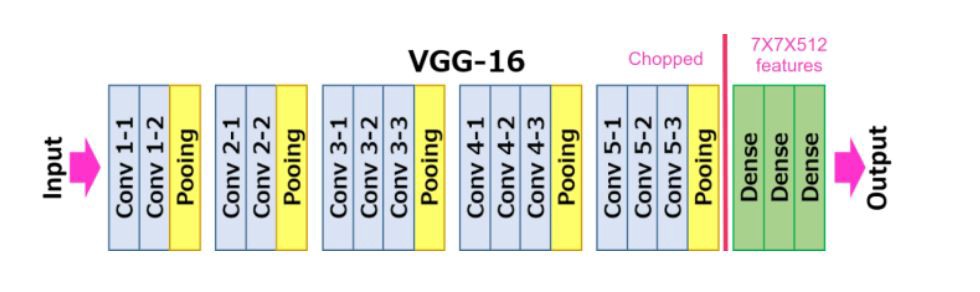
Source
To perform transfer learning import a pre-trained model using PyTorch, remove the last fully connected layer or add an extra fully connected layer in the end as per your requirement(as this model gives 1000 outputs and we can customize it to give a required number of outputs) and run the model.
Pre-processing
Preprocessing images before training is a very essential step to avoid errors. Preprocessing can resize the images to the same dimension and transform every image uniformly. different transformation tools available in torchvison.transforms is used for this process.
transform =   transforms.Compose([
        transforms.Resize((224, 224)),
        transforms.RandomHorizontalFlip(),
        transforms.ColorJitter(brightness=0.2, contrast=0.2, saturation=0.1, hue=0.1),
        transforms.RandomAffine(degrees=40, translate=None, scale=(1, 2), shear=15, resample=False, fillcolor=0),
        transforms.ToTensor(),
        transforms.Normalize((0.485, 0.456, 0.406), (0.229, 0.224, 0.225))
])
The images are loaded using ImageFolder and saved into a data loader. ImageFolder saves the images and their respective labels according to the folders they’re present in, and the dataloader divides the data into different batches for training. Here, a batch size of 8 is chosen.
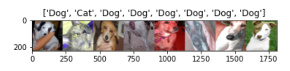
Visualising the dataset
Visualising the dataset before training the data is a good practice. This can be used to make sure data is loaded properly along with their labels and transformations are applied successfully.
For this process, the images are saved in a tensor format in a grid, and labels are extracted from the dictionary.
import torchvision
def imshow(inp, title=None):
    """Imshow for Tensor."""
    inp = inp.numpy().transpose((1, 2, 0))
    mean = np.array([0.485, 0.456, 0.406])
    std = np.array([0.229, 0.224, 0.225])
    inp = std * inp + mean
    inp = np.clip(inp, 0, 1)
    plt.imshow(inp)
    if title is not None:
        plt.title(title)
    plt.pause(0.001)  # pause a bit so that plots are updated
# Get a batch of training data
inputs, classes = next(iter(trainloader))
# Make a grid from batch
out = torchvision.utils.make_grid(inputs)
imshow(out,title=[class_names[x] for x in classes])
https://www.kaggle.com/tanayap2012/notebooka30b450d2f
Importing and training the model
The pre-trained model can be imported using Pytorch. The device can further be transferred to use GPU, which can reduce the training time.
import torchvision.models as models
device = torch.device("cuda" if torch.cuda.is_available() else "cpu")
model_ft = models.vgg16(pretrained=True)
The dataset is further divided into training and validation set to avoid overfitting. Some parameters used in this model while training is as follows:
- Criterion- Crossentropy loss
- optimiser- Stochastic gradient descent, learning rate=0.01, momentum=0.9
- Exponential Learning rate scheduler- This reduces the value of learning rate every 7 steps by a factor of gamma=0.1.
A linear fully connected layer is added in the end to converge the output to give two predicted labels.
num_ftrs = model_ft.fc.in_features
# Here the size of each output sample is set to 2.
# Alternatively, it can be generalized to nn.Linear(num_ftrs, len(class_names)).
model_ft.fc = nn.Linear(num_ftrs, 2)
#model_ft = model_ft.to(device)
criterion = nn.CrossEntropyLoss()
# Observe that all parameters are being optimized
optimizer_ft = optim.SGD(model_ft.parameters(), lr=0.001, momentum=0.9)
# Decay LR by a factor of 0.1 every 7 epochs
exp_lr_scheduler = lr_scheduler.StepLR(optimizer_ft, step_size=7, gamma=0.1)
These parameters can be chosen according to your own convenience and depending on the dataset.
Initially, we pass the inputs and labels to the model, and we get a predicted value of the label as an output. This predicted value and the actual value of the label are used to compute the cross-entropy loss, which is further used in backpropagation to update the value of weights and biases.
def train_model(model, criterion, optimizer, scheduler, num_epochs=25):
    since = time.time()
    best_model_wts = copy.deepcopy(model.state_dict())
    best_acc = 0.0
    for epoch in range(num_epochs):
        print('Epoch {}/{}'.format(epoch, num_epochs - 1))
        print('-' * 10)
        # Each epoch has a training and validation phase
        for phase in ['train', 'val']:
            if phase == 'train':
                model.train()  # Set model to training mode
            else:
                model.eval()   # Set model to evaluate mode
            running_loss = 0.0
            running_corrects = 0
            # Iterate over data.
            for inputs, labels in trainloader:
                inputs = inputs.to(device)
                labels = labels.to(device)
                # zero the parameter gradients
                optimizer.zero_grad()
                # forward
                # track history if only in train
                with torch.set_grad_enabled(phase == 'train'):
                    outputs = model(inputs)
                    _, preds = torch.max(outputs, 1)
                    loss = criterion(outputs, labels)
                    # backward + optimize only if in training phase
                    if phase == 'train':
                        loss.backward()
                        optimizer.step()
                # statistics
                running_loss += loss.item() * inputs.size(0)
                running_corrects += torch.sum(preds == labels.data)
            if phase == 'train':
                scheduler.step()
            epoch_loss = running_loss / dataset_sizes
            epoch_acc = running_corrects.double() / dataset_sizes
            print('{} Loss: {:.4f} Acc: {:.4f}'.format(
                phase, epoch_loss, epoch_acc))
            # deep copy the model
        print()
    time_elapsed = time.time() - since
    print('Training complete in {:.0f}m {:.0f}s'.format(
        time_elapsed // 60, time_elapsed % 60))
    # load best model weights
    model.load_state_dict(best_model_wts)
    return model
model_ft = train_model(model_ft, criterion, optimizer_ft, exp_lr_scheduler,
                       num_epochs=25)
After this step, you’ve successfully trained the model.
Thanks for reading!
The media shown in this article are not owned by Analytics Vidhya and are used at the Author’s discretion.


if i use "num_ftrs = model_ft.fc.in_features" at vgg16. It's not work. How i can solve this problem
num_ftrs = model_ft.classifier[6].in_features