Understand The DBSCAN Clustering Algorithm!

This article was published as a part of the Data Science Blogathon

Introduction

In this article, I’m gonna explain about DBSCAN algorithm. It is an unsupervised learning algorithm for clustering. First of all, I’m gonna explain every conceptual detail of this algorithm and then I’m gonna show you how you can code the DBSCAN algorithm using Sci-kit Learn.

The full name of the DBSCAN algorithm is Density-based Spatial Clustering of Applications with Noise. Well, there are three particular words that we need to focus on from the name. They are density, clustering, and noise. From the name, it is clear that the algorithm uses density to cluster the data points and it has something to do with the noise. Maybe it can identify the noise very well. We’ll see it later.

Table of Contents

1. What is density?
2. Important parameters of the DBSCAN algorithm
3. Classification of data points
4. Density edge and density connected points
5. Steps in the DBSCAN algorithm
6. How to determine epsilon and z?
7. Noise elimination
8. Practical
   implementation with Python

1. What is density?

First of all, let’s understand what is density.

Well from Physics we know that density is just the amount of matter present in a unit volume. We can easily extend this idea of volume into higher dimensions or even in a lower dimension.

For example, we have this region.

We have some data points in this region. And we have another region of the same area we have got these many data points here.

Source

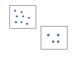
So, from the idea of density, the density of the first region is greater than the second region. Because, there are more data points, more matter in the first region. DBSCAN uses this concept of density to cluster the dataset. Now to understand the DBSCAN algorithm clearly, we need to know some important parameters.

2. Important parameters of the DBSCAN algorithm

The first one is epsilon.

2.1 Epsilon

It is a measure of the neighborhood.

What is a neighborhood?

2.2 Neighbourhood

Suppose, this is the point we are considering right now, and let me draw a circle around this point making this as a center and add a distance Epsilon.

So, we are gonna say this circle as this point’s neighborhood. So, epsilon is just a number that represents the radius of the circle around a particular point that we are going to consider the neighborhood of that point.

The next parameter is min_sample.

2.3 min_sample

I’m gonna represent min_samples as z throughout this article. If you gonna study this DBSCAN from some other sources then probably you may encounter this term min_samples or minPts and so on. This is a threshold on the least number of points that we want to see in a point’s neighborhood. Suppose we are
taking z = 3.

Source

If we have 4 points in our neighborhood, this will also satisfy our threshold z = 3. Because this threshold represents the minimum number of samples in a neighborhood.

3. Classification of data points

Now based on these two parameters i.e., epsilon and min_samples, we are first going to classify every point in our dataset into three categories. They are

• Core points
• Boundary points or border points
• Noise points

Let’s see the core points first.

3.1 Core points

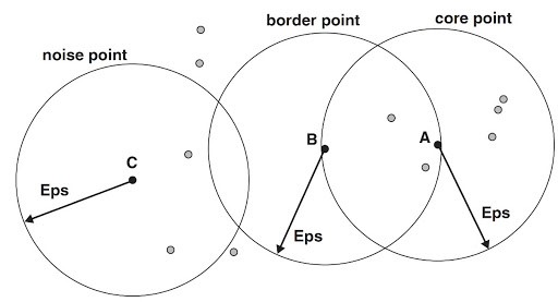
Now see the above-mentioned figure. I represented a core point A.

If I say a point as a core point then it must satisfy one condition. The condition is the number of neighbors must be greater than or equal to our threshold min_samples or z. If I set z = 3, then this point satisfies this condition. Hence, we say this is the core point.

Let’s see the second type of point.

3.2 Boundary points

If I say one point as a boundary point, then it has to satisfy the following two conditions.

• The number of neighbors must be less than z.
• The point should be in the neighborhood of a core point.

Consider the same figure mentioned above. I represented a border point B. The point has less than the number of neighbors in its neighborhood and it is in the neighborhood of another core point. So, this point B is a boundary point or border point.

Now let’s see the last kind of points.

3.3 Noise points

The definition of noise point is very simple. If a point is neither a core point nor a boundary point, then it is called a noise point. In the above-mentioned figure, point C is neither a core point nor a boundary point. So, we can say that as a noise point.

Now we have classified every single data point into three categories. This is the first step in the DBSCAN algorithm.

Now you need to understand another concept.

4. Density edge and density connected points

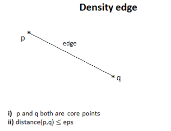
4.1 Density edge

Suppose we have got
two core points. If two points are neighbors then we join them by an edge that
we call a density edge.

Source

4.2 Density connected points

Let’s consider 6 points. Let me assume that every point is a core point. Assume they are connected
via density edges.

Source

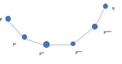
You can see that p’ is in the neighborhood of p” and similarly for other points. But p and q are not neighbors. If this kind of situation arises, when two core points are connected via density edges, then we say p and q are density connected points.

Now let’s see the steps of this algorithm.

5. Steps in the DBSCAN algorithm

1. Classify the points.

2. Discard noise.

3. Assign cluster to a core point.

4. Color all the density connected points of a core point.

5. Color boundary points according to the nearest core point.

The first step is already explained above.

The second is just eliminating the noise points.

Let’s see about the third step. For example, I am taking a core point and assigning it a cluster red. In the fourth step, we have to color all the density-connected points to the selected core point in the third step, the color red. Remember here, we should not color boundary points.

We have to repeat the third and fourth steps for every uncolored core point.

The DBSCAN algorithm is done!

Let me explain a couple of very important points about this algorithm.

6. How to determine epsilon and z?

To be honest this is a difficult question because the DBSCAN algorithm is very sensitive to its initial parameters. So, if you change the values of epsilon and z even slightly, then your algorithm can produce very different results. This is one downside of this algorithm. But you can choose those values wisely if you have the proper domain knowledge. As a rule of thumb, if you have a large number of examples then you can choose z in the order of your dimensionality. If you are working with 10 dimensionalities then it is preferable to choose a value of z close to 10 like 12 or 15.

Now to know the value of epsilon, here is a thing you can try. Suppose you have chosen z = 5. So, after that what you will do? You will find the distance of the 5^th neighbor from every data point.

So, you will have a distance array and the i^th entry in that array will represent the distance of the 5^th neighbor of the i^th data point. And then you are gonna sort this distance array and you are gonna plot it like this. On the y axis, you will just have the distance and on the x-axis, you will have the index (i).

Ideally, you should get a graph like this.

Source

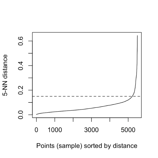
As we have sorted this, as the index will increase the distance of the 5^th data point from that point will also increase. If your luck favors, you can find this elbow type of thing. You can cut that by a horizontal line and the horizontal line will cut the y-axis at some point and you can just take this value as your epsilon. But in the real world, you might not get this smooth elbow. But this is the trick that can be applied in some cases.

Now let me come to the second important point.

7. Noise elimination

DBSCAN is very effective in noise elimination.

As you saw in my previous example, we were classifying the points into three categories and there was a category of noise points. So, this algorithm can be applied in noisy datasets very well. And the last point is DBSCAN can’t handle higher dimensional data very well. This is a fault of many clustering algorithms. As the dimensionality increases, we have to look into a larger volume to find the same number of neighbors. So, the similarity between the points decreases. That will result in clustering errors.

Now let’s jump into the code section.

8. Practical implementation with Python

First of all, I’m gonna make a fake dataset. To make a fake dataset, we are using our favorite library Sci-kit Learn. We need to import the function called make_blobs from sklearn.datasets.

The function takes n_samples which represents how many data points we need to produce.

And the second argument centers. This tells us that how many clusters will be there.

The third argument n_features is just the dimensionality of our dataset.

random_state is used to produce the same results. This function will return two things.

The first one is the data points that I am assigning to the variable X and the second thing is it will return an array of labels.

Now, remember that DBSCAN is unsupervised learning. So, we don’t provide the labels i.e., the ground truth at the beginning. We let our algorithm find those labels on its own. We need some other libraries like
pandas, matplotlib, and NumPy.
Moving on with visualization you can see that we have got three clusters here. Now our DBSCAN algorithm will try to find the labels on its own.

Python Code:

DBSCAN algorithm is really simple to implement in python using scikit-learn. The class name is DBSCAN. We need to create an object out of it. The object here I created is clustering. We need to input the two most
important parameters that I have discussed in the conceptual portion. The first one epsilon eps and the second one is z or min_samples. Now I have given epsilon as 1 and min_samples as 5. We are just getting the labels of the clusters in the next step.

from sklearn.cluster import DBSCAN
clustering = DBSCAN(eps = 1, min_samples = 5).fit(X)
cluster = clustering.labels_

To see how many clusters has it found on the dataset, we can just convert this array into a set and we can print the length of the set. Now you can see that it is 4.

len(set(cluster))

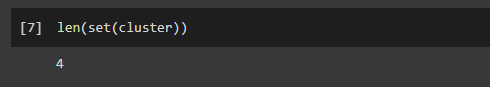
But what happened?

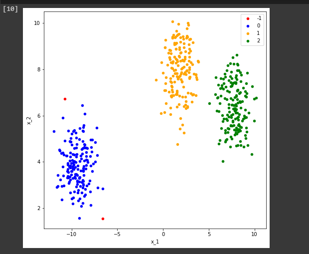
We saw that our dataset contains three clusters.

The first cluster that is the -1 level represents the noise in this DBSCAN. You can see we just visualize our clusters by this simple piece of code then we will find something like this.

def show_clusters(X, cluster):
  df = DataFrame(dict(x=X[:,0], y=X[:,1], label=cluster))
  colors = {-1: 'red', 0: 'blue', 1:'orange', 2:'green', 3:'yellow'}
  fig, ax = plt.subplots(figsize=(8,8))
  grouped = df.groupby('label')
  for key, group in grouped:
    group.plot(ax=ax, kind='scatter', x='x', y='y', label=key, color=colors[key])
  plt.xlabel('x_1')
  plt.ylabel('x_2')
  plt.show()

show_clusters(X, cluster)

So, that’s how easy it is to implement DBSCAN using sci-kit learn.

Endnotes

I hope you are now convinced to apply the DBSCAN on some datasets. It’s time to get your hands on
it!

The media shown in this article are not owned by Analytics Vidhya and are used at the Author’s discretion.