A walkthrough of Univariate Anomaly Detection in Python

This article was published as a part of the Data Science Blogathon

Introduction to Anomaly Detection

An anomaly is an observation that deviates significantly from all the other observations. An anomaly detection system is a system that detects anomalies in the data. An anomaly is also called an outlier.

Example: Let’s say a column of data consists of the income of citizens per month and that column contains the salary of Bill Gates as well. Then the salary of Bill Gates is an outlier in this data.

Anomaly Detection Algorithms

In this blog, let us go through the following anomaly detection algorithms.

• Interquartile Range

• Isolation Forest

• Median Absolute Deviation

• K-Nearest Neighbours

These are a few of the many algorithms available and never hold back yourself from exploring more algorithms other than these.

Import the required libraries and write the utility functions

# python outlier detection
!pip install pyod

import warnings
import numpy as np
import pandas as pd
from pyod.models.mad import MAD
from pyod.models.knn import KNN
from pyod.models.lof import LOF
import matplotlib.pyplot as plt
from sklearn.ensemble import IsolationForest

# data for anomaly detection
data_values = [['2021-05-1', 45000.0],
       ['2021-05-2', 70000.0],
       ['2021-05-3', 250000.0],
       ['2021-05-4', 70000.0],
       ['2021-05-5', 45000.0],
       ['2021-05-6', 55000.0],
       ['2021-05-7', 35000.0],
       ['2021-05-8', 60000.0],
       ['2021-05-9', 45000.0],
       ['2021-05-10', 25000.0],
       ['2021-05-11', 142936.0],
       ['2021-05-12', 138026.0],
       ['2021-05-13', 28347.0],
       ['2021-05-14', 40962.66],
       ['2021-05-15', 34543.0],
       ['2021-05-16', 40962.66],
       ['2021-05-17', 25207.0],
       ['2021-05-18', 37502.0],
       ['2021-05-19', 29589.0],
       ['2021-05-20', 78404.0],
       ['2021-05-21', 26593.0],
       ['2021-05-22', 123267.0],
       ['2021-05-23', 46880.0],
       ['2021-05-24', 65361.0],
       ['2021-05-25', 46042.0],
       ['2021-05-26', 48209.0],
       ['2021-05-27', 44461.0],
       ['2021-05-28', 90866.0],
       ['2021-05-29', 46886.0],
       ['2021-05-30', 33456.0],
       ['2021-05-31', 46251.0],
       ['2021-06-1', 29370.0],
       ['2021-06-2', 165620.0],
       ['2021-06-3', 20317.0]]
       
data = pd.DataFrame(data_values , columns=['date', 'amount'])

def fit_model(model, data, column='amount'):
    # fit the model and predict it
    df = data.copy()
    data_to_predict = data[column].to_numpy().reshape(-1, 1)
    predictions = model.fit_predict(data_to_predict)
    df['Predictions'] = predictions
    
    return df

def plot_anomalies(df, x='date', y='amount'):

    # categories will be having values from 0 to n
    # for each values in 0 to n it is mapped in colormap
    categories = df['Predictions'].to_numpy()
    colormap = np.array(['g', 'r'])

    f = plt.figure(figsize=(12, 4))
    f = plt.scatter(df[x], df[y], c=colormap[categories])
    f = plt.xlabel(x)
    f = plt.ylabel(y)
    f = plt.xticks(rotation=90)
    plt.show()

Hit Run to see the output

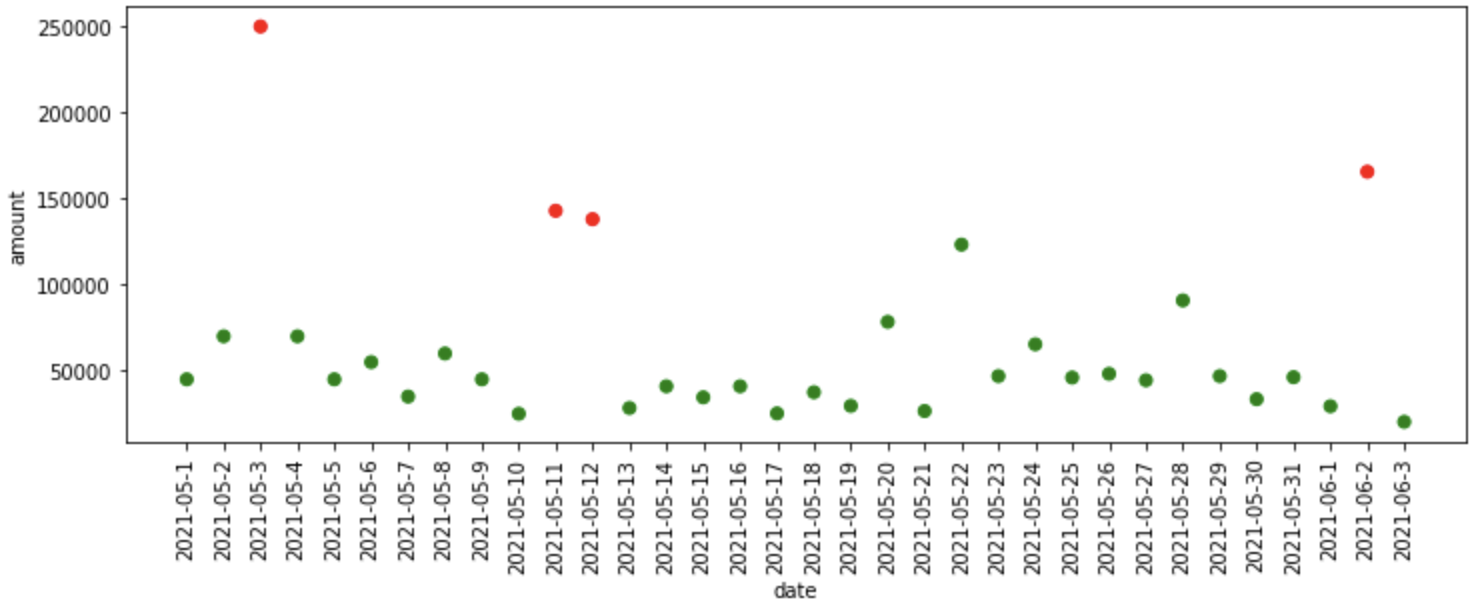
The data above consists of two columns namely date and amount, we can assume that the data contains the sales amount of a bakery showcase company.

What does the fit_model function do?

• The fit_model function takes in model and data as input, here we are finding anomalies on the amount column.
• After that, it reshapes the data into one-dimensional data and fits the provided model and predicts the anomalies in the data and stores it in the predictions column of the provided data frame, and returns it.

Interquartile Range

Percentiles:

• nth percentile denotes that ‘n’ percentage of values would fall below the nth percentile.

• Example: Consider the following example in which there are 20 random numbers

  • 5, 7, 10, 15, 21, 24, 31, 32, 39, 45, 46, 49, 52, 57, 59, 62, 72, 87, 92, 100

  • The 25th percentile of the above list is 23.25, below which 25% of values fall (25% * 20 = 5).

  • The 50th percentile of the above list is 45.50, below which 50% of values fall (50% * 20 = 10 ).

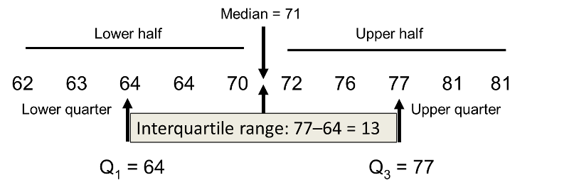
Quartiles:

• 1st Quartile = 25th percentile

• 2nd Quartile = 50th percentile

• 3rd Quartile = 75th percentile

Interquartile Range (IQR):

IQR = 3rd Quartile – 1st Quartile

Anomalies = [1st Quartile – (1.5 * IQR)] or [3rd Quartile + (1.5 * IQR)]

Anomalies lie below [1st Quartile – (1.5 * IQR)] and above [3rd Quartile + (1.5 * IQR)] these values.

Image Source

def find_anomalies(value, lower_threshold, upper_threshold):
    
    if value < lower_threshold or value > upper_threshold:
        return 1
    else: return 0

def iqr_anomaly_detector(data, column='amount', threshold=1.1):
    
    df = data.copy()
    quartiles = dict(data[column].quantile([.25, .50, .75]))
    quartile_3, quartile_1 = quartiles[0.75], quartiles[0.25]
    iqr = quartile_3 - quartile_1

    lower_threshold = quartile_1 - (threshold * iqr)
    upper_threshold = quartile_3 + (threshold * iqr)

    print(f"Lower threshold: {lower_threshold}, \nUpper threshold: {upper_threshold}\n")
    
    df['Predictions'] = data[column].apply(find_anomalies, args=(lower_threshold, upper_threshold))
    return df
  
iqr_df = iqr_anomaly_detector(data)
plot_anomalies(iqr_df)
# output
# Lower threshold: -2944.050000000003, 
# Upper threshold: 106441.55

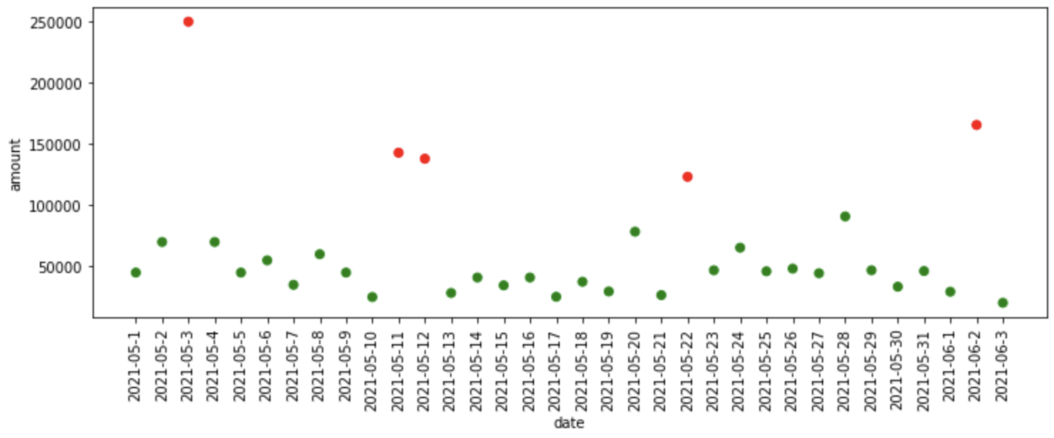
What happened in the code above?

• First of all, it finds out the 25th and 75th percentile, in other words, 1st and 3rd quartile were found.
• And then, the interquartile range is found which is the difference between the third and first quartile.
• After that, we are finding the upper and lower threshold above and below which the anomalies lie respectively.
• The find_anomalies function above finds the anomalies in the data according to the thresholds provided.
• Finally, we are plotting the anomalies found.

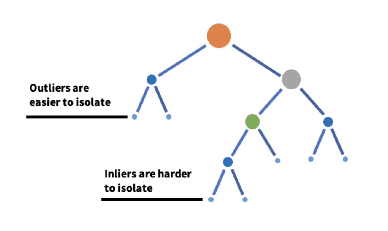
Isolation Forest

Isolation Forest is an algorithm that detects anomalies by taking a subset of data and constructing many isolation trees out of it.

• The core idea is that the anomalies are much easier to isolate than the normal observations and the anomalies exist in much smaller depths of an isolation tree. An isolation tree is constructed by randomly selecting a feature and randomly selecting a value from that feature. A forest is constructed by aggregating all the isolation trees.

Image Source

iso_forest = IsolationForest(n_estimators=125)
iso_df = fit_model(iso_forest, data)
iso_df['Predictions'] = iso_df['Predictions'].map(lambda x: 1 if x==-1 else 0)
plot_anomalies(iso_df)

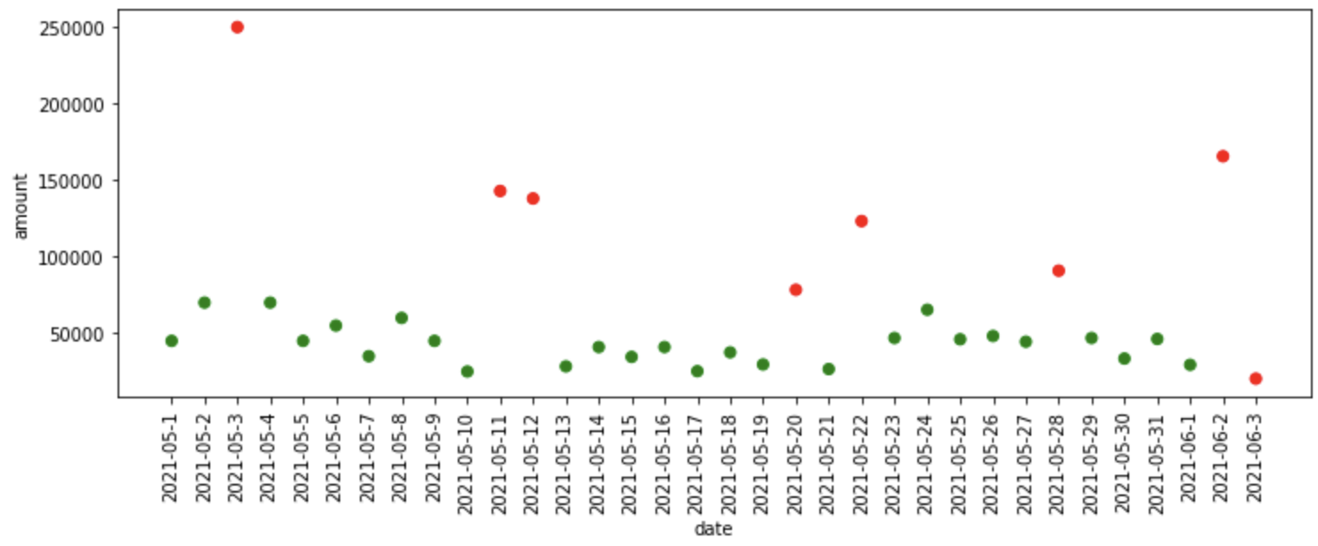
What happened in the code above?

• First, we define the Isolation Forest model with 125 isolation trees, then we pass the model, data as inputs to the fit_model function, where it fits the model on the data and provides predictions to us.
• The isolation forest assigns -1 to the anomalous data and 1 to the normal data, so for simplicity, we convert the normal data prediction (1) to 0 and anomalous data prediction(-1) to 1.
• Finally, we plot the anomalies predicted by Isolation Forest.

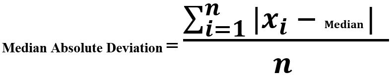
Median Absolute Deviation

Median Absolute Deviation is the difference between each observation and the median of those observations. An observation that deviates more from the rest of the observation is considered to be an anomaly.

Why median rather than mean?

• The computation of mean is highly influenced by the outliers and a mean value would be spurious if there are outliers in data.

 

"""Median Absolute Deviation"""
mad_model = MAD()
mad_df = fit_model(mad_model, data)
plot_anomalies(mad_df)

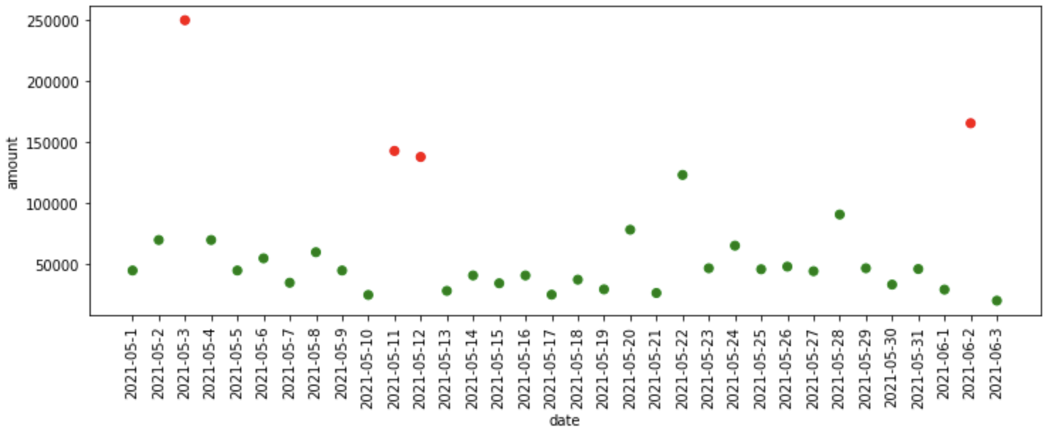
What happened in the code above?

• First, we define the Median Absolute Deviation model which is available in pyod library, then we pass the model, data as inputs to the fit_model function, where it fits the model on the data and provides predictions to us.
• Finally, we plot the anomalies predicted by MAD model.

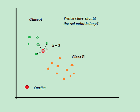
K-Nearest Neighbours algorithm

K-Nearest Neighbours algorithm detects anomalies using the distances of k-nearest neighbors as anomaly scores. The idea is that if an observation is much far from the other observations then that observation is considered to be an anomaly.

"""KNN Based Outlier Detection"""
knn_model = KNN()
knn_df = fit_model(knn_model, data)
plot_anomalies(knn_df)

What happened in the code above?

• First, we define the K-Nearest Neighbour model which is available in pyod library, then we pass the model, data as inputs to the fit_model function, where it fits the model on the data and provides predictions to us.
• Finally, we plot the anomalies predicted by the KNN model.

There are a plethora of models available in the PyOD library like,

• CBLOF (Cluster Based Local Outlier Factor)
• LOF (Local Outlier Factor)
• HBOS (Histogram Based Outlier Detection)
• OCSVM (One class SVM)

Never hold yourself back from experimenting with more algorithms available in PyOD.

The practical implementations of the above algorithms are implemented in the following notebook

Google Colaboratory Link

References

[1] PyOD, Python Outlier Detection library

Thank you!

The media shown in this article are not owned by Analytics Vidhya and are used at the Author’s discretion.