This article was published as a part of the Data Science Blogathon
This article would try to make an effort to take the deepest possible plunge in the ocean of deep learning. Mariana Trench is the deepest trench on earth located in the pacific ocean, so in the ocean of deep learning, we shall try to reach as close to the Mariana Trench. This is a continuation of the previous article, the link of which has been shared below for reference-
https://www.analyticsvidhya.com/blog/2021/07/plunging-into-deep-learning-carrying-a-red-wine/
This article would cover overfitting and underfitting, and drop out and batch normalization using ‘heart dataset’. The dataset can be downloaded for reference using the following link-
https://www.kaggle.com/ronitf/heart-disease-uci
Introduction
Underfitting and Overfitting – Taking care of underfitting and overfitting enable performance enhancement either by adding capacity or stopping early.
Dropout and Normalization – Take care of underfitting and overfitting. So, let’s discuss the two very important concepts.
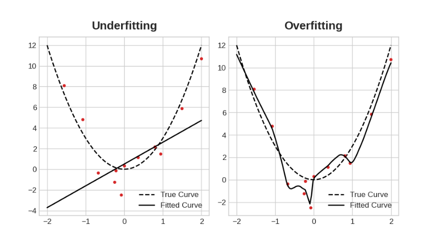
Underfitting and Overfitting
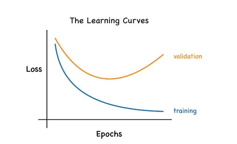
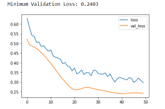
The above image represents validation loss which gives an idea of an unseen error on invisible data. During the training of a model, the loss on the training set is plot epoch by epoch. To this, we have added another parameter validation data. The condition in which the training loss will go down when the model learns signal or it learns noise. For a nearly ideal situation, the model needs a negotiation with the signal as well as noise which is not enough the signal and not enough noise.
Criteria for underfitting and Overfitting
1. Underfitting when the loss of signal is not very low as the model has not learned enough signal.
2. Overfitting when the loss of signal is not very low as the model has learned enough too much noise.
Method’s to reduce the amount of noise and to get more signal out of training data
1. Capacity – It is the ability of the model to learn the size as well as the complexity of patterns.
2. Early stopping – When the model learns noise too eagerly, the validation loss also starts to increase. Stopping the training to prevent further validation loss, early stopping is applied.
Minutes of the concepts would be better comprehended with the help of the lines of code that follows along with the outputs.
import pandas as pd
Cardiology = pd.read_csv('heart.csv')
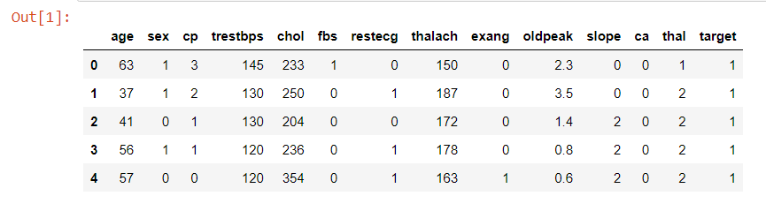
Cardiology.head()
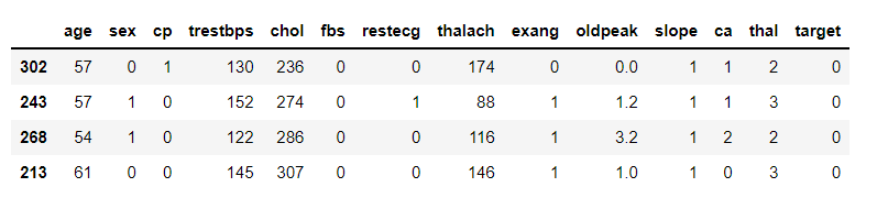
df_train = Cardiology.sample(frac=0.7, random_state=5)
df_valid = Cardiology.drop(df_train.index)
display(df_train.head(4))
max_ = df_train.max(axis=0)
min_ = df_train.min(axis=0)
df_train = (df_train - min_) / (max_ - min_)
df_valid = (df_valid - min_) / (max_ - min_)
X_train = df_train.drop('target', axis=1)
X_valid = df_valid.drop('target', axis=1)
y_train = df_train['target']
y_valid = df_valid['target']
input_shape = [X_train.shape[1]]
print("Input shape: {}".format(input_shape))

from tensorflow import keras
from tensorflow.keras import layers
from tensorflow.keras import callbacks
model = keras.Sequential([
layers.Dense(1, input_shape=input_shape),
])
model.compile(
optimizer='adam',
loss='mae',
)
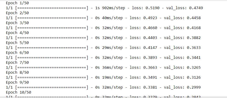
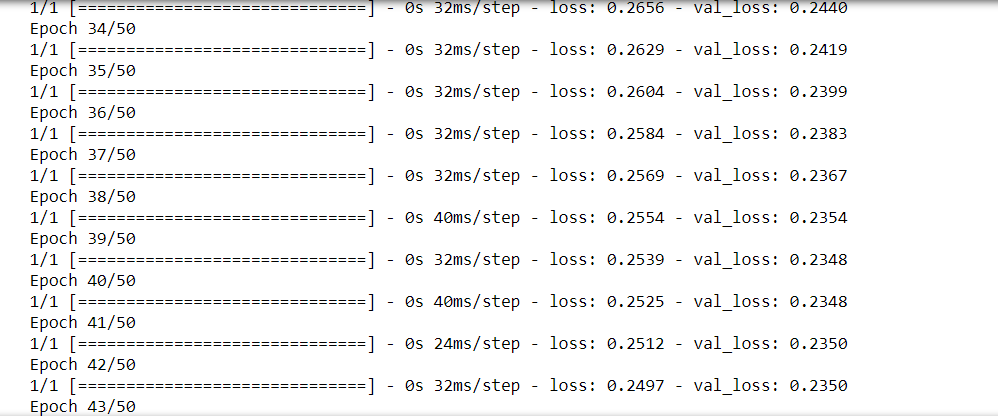
history = model.fit(
X_train, y_train,
validation_data=(X_valid, y_valid),
batch_size=512,
epochs=50,
verbose=0,
)
history_df = pd.DataFrame(history.history)
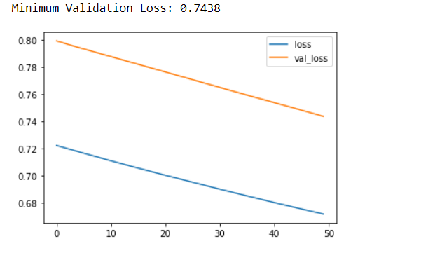
history_df.loc[0:, ['loss', 'val_loss']].plot()
print("Minimum Validation Loss: {:0.4f}".format(history_df['val_loss'].min()));
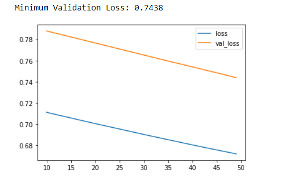
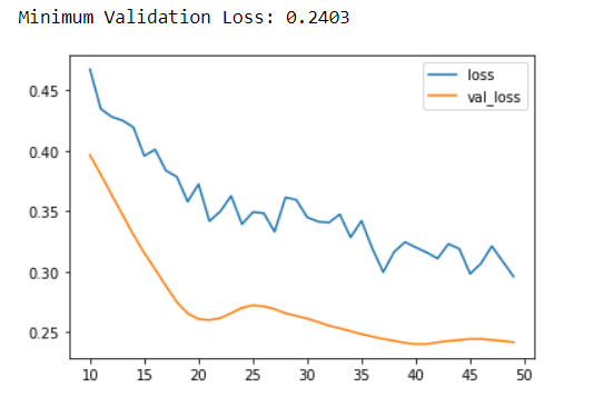
history_df.loc[10:, ['loss', 'val_loss']].plot()
print("Minimum Validation Loss: {:0.4f}".format(history_df['val_loss'].min()));
model = keras.Sequential([
    layers.Dense(128, activation='relu', input_shape=input_shape),
    layers.Dense(64, activation='relu'),
    layers.Dense(1)
])
model.compile(
    optimizer='adam',
    loss='mae',
)
history = model.fit(
    X_train, y_train,
    validation_data=(X_valid, y_valid),
    batch_size=512,
    epochs=50,
)
history_df = pd.DataFrame(history.history)
history_df.loc[:, ['loss', 'val_loss']].plot()
print("Minimum Validation Loss: {:0.4f}".format(history_df['val_loss'].min()));
from tensorflow.keras.callbacks import EarlyStopping
early_stopping = EarlyStopping(
                min_delta=0.001,patience=5,restore_best_weights=True,)
model = keras.Sequential([
    layers.Dense(128, activation='relu', input_shape=input_shape),
    layers.Dense(64, activation='relu'),
    layers.Dense(1)
])
model.compile(
    optimizer='adam',
    loss='mae',
)
history = model.fit(
    X_train, y_train,
    validation_data=(X_valid, y_valid),
    batch_size=512,
    epochs=50,
    callbacks=[early_stopping]
)
history_df = pd.DataFrame(history.history)
history_df.loc[:, ['loss', 'val_loss']].plot()
print("Minimum Validation Loss: {:0.4f}".format(history_df['val_loss'].min()));
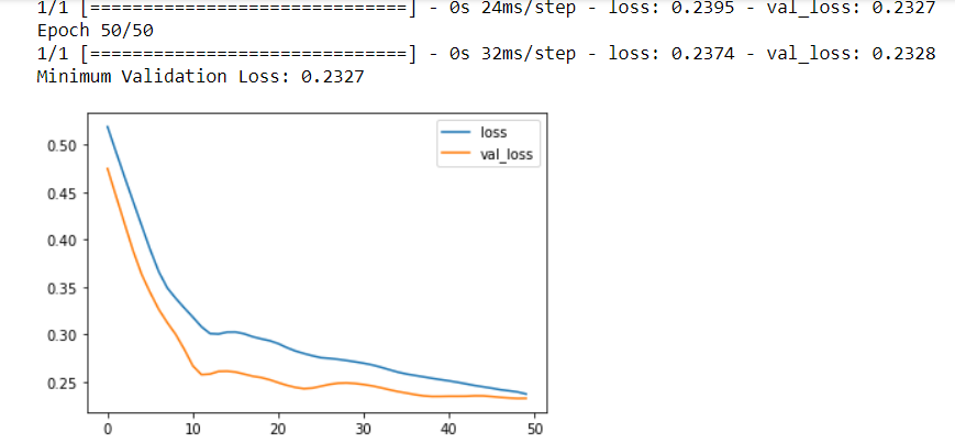
At the outset, we have loaded the dataset. The dataset was then split into the training part and the testing part. The target is the output variable and the rest 13 are all input variables. In the next step, we imported keras, layers, and callback from tensorflow. After importing the necessary libraries and modules, we have started by training a low-capacity linear model. In the output, we can see a huge gap between the loss and the validation loss curve, indicating that the network is overfitting.
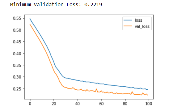
After that, we have added capacity to the network by incorporating 3 hidden layers with each having a unit value of 128. We can observe that validation loss and training loss have begun to come very close. So, this suggests that the network is about to underfit.
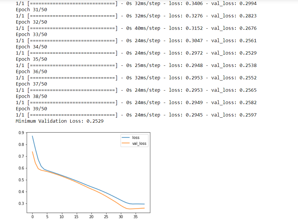
At this point, we define early stopping callback with patience = 5 epochs, change in validation loss, min_delta=0.001, and setting restore_best_weights=True. In the output, we observed that the early stopping callback stopped the training once the network began underfitting. In addition, with the inclusion of restore_best_weights, the model could be kept where the validation loss was lowest.
Dropout and Batch Normalization
Beyond dense layers, there exist special layers too. Dropout and Batch Normalization are 2 special types of layers. On their own, these layers do not contain any neurons but add valuable functionalities which are beneficial for the model.
1.Dropout– It can rectify overfitting. Overfitting results in spurious patterns in the training data, so to detect these, the network relies on specific combinations of weight. This is also known as conspiracies of weight. The dropout helps in removing such conspiracies by dropping out some fraction of the layer’s input units during each step of training.
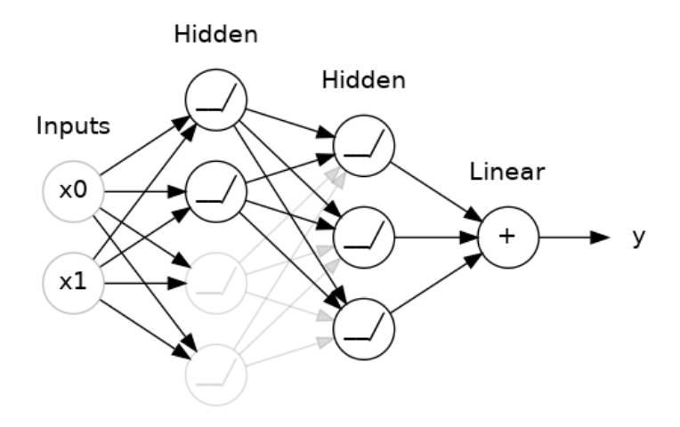
In the above image, 50% dropout addition has taken place between 2 hidden layers.
2. Batch Normalization – It enables to rectify the training that is either slow or not stable. For convenience, it is important to put all the data on a common scale-like scikit-learn’s StandardScaler as SGD(Stochastic Gradient Descent) shifts the network weights in sync with the largeness of the activation the data produces. A batch normalization layer allows us to do this inside the network by looking at each batch as it comes in.
Initially, the batch gets normalized with its own mean and standard deviation. Then, the data are being put on a new scale. It can be used at almost any point in the network.
Minutes of the concepts would be better comprehended with the help of the lines of code that follows along with the outputs.
model = keras.Sequential([
    layers.Dense(128, activation='relu', input_shape=input_shape),
    layers.Dropout(0.3),
    layers.Dense(64, activation='relu'),
    layers.Dropout(0.3),
    layers.Dense(1)
])
model.compile(
    optimizer='adam',
    loss='mae',
)
history = model.fit(
    X_train, y_train,
    validation_data=(X_valid, y_valid),
    batch_size=512,
    epochs=50,
    verbose=0
)
history_df = pd.DataFrame(history.history)
history_df.loc[0:, ['loss', 'val_loss']].plot()
print("Minimum Validation Loss: {:0.4f}".format(history_df['val_loss'].min()));
history_df.loc[10:, ['loss', 'val_loss']].plot()
print("Minimum Validation Loss: {:0.4f}".format(history_df['val_loss'].min()));
In the heart model, we have added 2 dropout layers. The layers have been added one each after the Dense layer with 128 units and another Dense layer with 64 units. The drop-out rate in both cases has been set to 0.3. Now, we have run lines of code that are exactly similar to the one we ran previously where the model tended to overfit the data. Here, the addition of dropout seems to have helped in closing the gap.
model = keras.Sequential([
    layers.Dense(512, activation='relu', input_shape=input_shape),
    layers.Dense(512, activation='relu'),
    layers.Dense(512, activation='relu'),
    layers.Dense(1),
])
model.compile(
    optimizer='sgd', # SGD is more sensitive to differences of scale
    loss='mae',
    metrics=['mae'],
)
history = model.fit(
    X_train, y_train,
    validation_data=(X_valid, y_valid),
    batch_size=64,
    epochs=100,
    verbose=0,
)
history_df = pd.DataFrame(history.history)
history_df.loc[0:, ['loss', 'val_loss']].plot()
print(("Minimum Validation Loss: {:0.4f}").format(history_df['val_loss'].min()))
This dataset got trained properly, so did manifest with a minimum validation loss. A certain dataset will fail the training of this network. Let’s try with ‘spotify’ dataset. The link can be found below-
model = keras.Sequential([
    layers.Dense(512, activation='relu', input_shape=input_shape),
    layers.Dense(512, activation='relu'),
    layers.Dense(512, activation='relu'),
    layers.Dense(1),
])
model.compile(
    optimizer='sgd', # SGD is more sensitive to differences of scale
    loss='mae',
    metrics=['mae'],
)
history = model.fit(
    X_train, y_train,
    validation_data=(X_valid, y_valid),
    batch_size=64,
    epochs=100,
    verbose=0,
)
history_df = pd.DataFrame(history.history)
history_df.loc[0:, ['loss', 'val_loss']].plot()
print(("Minimum Validation Loss: {:0.4f}").format(history_df['val_loss'].min()))
In this dataset, training the dataset failed as it is converging to a very large network. Here, the role of batch normalization becomes very prominent.
model = keras.Sequential([
     layers.BatchNormalization(),
    layers.Dense(512, activation='relu', input_shape=input_shape),
     layers.BatchNormalization(),
    layers.Dense(512, activation='relu'),
     layers.BatchNormalization(),
    layers.Dense(512, activation='relu'),
     layers.BatchNormalization(),
    layers.Dense(1),
])
model.compile(
    optimizer='sgd',
    loss='mae',
    metrics=['mae'],
)
EPOCHS = 100
history = model.fit(
    X_train, y_train,
    validation_data=(X_valid, y_valid),
    batch_size=64,
    epochs=EPOCHS,
    verbose=0,
)
history_df = pd.DataFrame(history.history)
history_df.loc[0:, ['loss', 'val_loss']].plot()
print(("Minimum Validation Loss: {:0.4f}").format(history_df['val_loss'].min()))
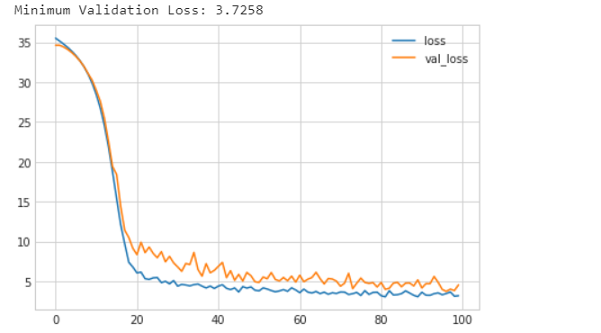
We have added 4 BatchNormalization layers preceding the dense layers. It could be concluded that the addition of batch normalization layers helped to adaptively scale the data while passing through the network. On a difficult dataset, unlike the heart dataset, batch normalization can prove to be an asset.
Conclusion
Deep learning is a key component of Artificial Intelligence and has the potential to overhaul many aspects of life including the medical and healthcare sectors. This article covered most of the important concepts of deep learning shortly and crisply. Practicing with the different datasets is important to learn deeper.
Thanks a lot for going through this article. I hope this article did add value to the time you have devoted!
References
1. Holbrook, R.(n.d). Kaggle. Intro to Deep Learning. Retrieved from https://www.kaggle.com
The media shown in this article are not owned by Analytics Vidhya and are used at the Author’s discretion.
I am a biotechnology graduate with experience in Administration, Research and Development, Information Technology & management, and Academics of more than 12 years. I have experience of working in organizations like Ranbaxy, Abbott India Limited, Drivz India, LIC, Chegg, Expertsmind, and Coronawhy.
Recognition:
1. Played major role in making a brand “Duphaston” worth “Rs 100 crores INR” in Abbott India Limited as Therapy Business Manager of Women’s health and gastro intestine team.
2. Won “best marketing skills” award in Abbott India Limited.
3. Came on the merit list of National IT aptitude test, 2010.
4. Represented my school in regional social science exhibition.
Courses and Trainings:
1. Took 54 hours training on vb.net in Niit, Guwahati.
2. Underwent training of 7 days on targeting and segmentation in Abbott India ltd, Lonavala.
3. Earned “Elite Certificate” from IIT-Madras on “Python for Data Science”.


