This article was published as a part of the Data Science Blogathon
Introduction
One of my last articles was all about Convolutional Network, Its working and components. We also saw a simple implementation of CNN in Python. In this article, we will perform Image Classification using a Convolutional Neural Network and learn about all the steps in detail. So if you are new to this then keep on reading.
To give you a brief, CNN is a deep learning algorithm and one of the types of Neural networks which works for images and videos. There are various things we can achieve from CNN, some of them are Image classification, Image recognition, Object Detection, Face recognition, and many more.
Today, we will perform Image classification on the CIFAR10 Dataset which is a part of the Tensorflow library. It consists of images of various objects such as ships, frogs, aeroplanes, dogs, automobiles. The dataset has a total of 60,000 coloured images and 10 labels. Let’s jump into the coding part now.
Implementation
# importing necessary libraries
import numpy as np
import matplotlib.pyplot as plt
%matplotlib inline
# To convert to categorical data
from tensorflow.keras.utils import to_categorical
#libraries for building model
from tensorflow.keras.models import Sequential
from tensorflow.keras.layers import Dense, Conv2D, MaxPool2D, Dropout,Flatten
from tensorflow.keras.datasets import cifar10
#loading the data
(X_train, y_train), (X_test, y_test) = cifar10.load_data()
Exploratory Data Analysis
#shape of the dataset
print(X_train.shape)
print(y_train.shape)
print(X_test.shape)
print(y_test.shape)
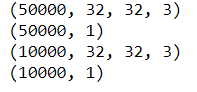
Our train data has 50,000 images and test data has 10,000 images of size 32*32 and 3 channels i.e RGB (Red, Green, Blue)
#checking the labels
np.unique(y_train)

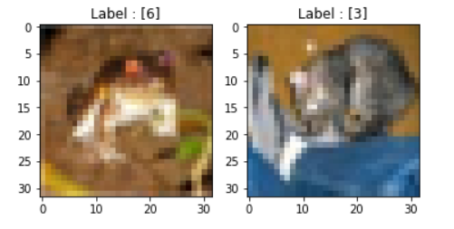
#first image of training data
plt.subplot(121)
plt.imshow(X_train[0])
plt.title("Label : {}".format(y_train[0]))
#first image of test data
plt.subplot(122)
plt.imshow(X_test[0])
plt.title("Label : {}".format(y_test[0]));
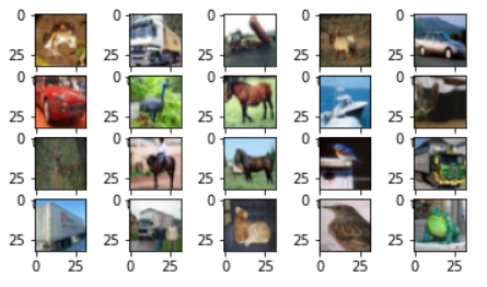
#visualizing the first 20 images in the dataset
for i in range(20):
    #subplot
    plt.subplot(5, 5, i+1)
    # plotting pixel data
    plt.imshow(X_train[i], cmap=plt.get_cmap('gray'))
# show the figure
plt.show()
Preprocessing Data
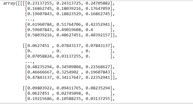
For data preprocessing we just need to perform two steps here, first is scaling the pixel values of images between 0 to 1, and the second is reshaping the labels to 1D from 2D
# Scale the data to lie between 0 to 1
X_train = X_train/255
X_test = X_test/255
print(X_train)
#reshaping the train and test lables to 1D
y_train = y_train.reshape(-1,)
y_test = y_test.reshape(-1,)
We can see in the above figure that the pixel values of images have been scaled between 0 to 1 and labels have also been reshaped. The data is ready for modelling so let’s build the CNN Model now.
Model Building
As we discussed earlier that a Deep Learning model is built in 5 steps i.e Defining the model, Compiling the model, Fitting the model, Evaluation the model, and Making Predictions, that’s what we are going to do here as well.
Step 1: Defining the model
model=Sequential()
#adding the first Convolution layer
model.add(Conv2D(32,(3,3),activation='relu',input_shape=(32,32,3)))
#adding Max pooling layer
model.add(MaxPool2D(2,2))
#adding another Convolution layer
model.add(Conv2D(64,(3,3),activation='relu'))
model.add(MaxPool2D(2,2))
model.add(Flatten())
#adding dense layer
model.add(Dense(216,activation='relu'))
#adding output layer
model.add(Dense(10,activation='softmax'))
We have added the first Convolution layer with 32 filters of size (3*3), the activation function used is Relu, and provided the input shape to the model.
Next added the Max Pooling layer of size (2*2). Max pooling helps in reducing dimensions. Please refer to the CNN article for an explanation of CNN components.
Then we have added one more Convolution layer with 64 filters of size (3*3) and a Max Pooling layer of size (2*2)
In the next step, we Flattened the layers to pass them onto the Dense layer and added a Dense layer of 216 neurons.
At last, the output layer is added with a softmax activation function as we have 10 labels.
Step 2: Compiling the model
model.compile(optimizer='rmsprop',loss='sparse_categorical_crossentropy',metrics=['accuracy'])
Step 3: Fitting the model
model.fit(X_train,y_train,epochs=10)

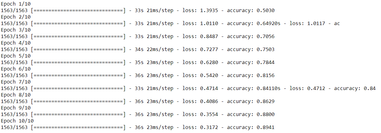
As seen in the above figure we have got an accuracy of 89% and loss is 0.31. Let’s see the accuracy of test data.
Step 4: Evaluating the model
model.evaluate(X_test,y_test)

The accuracy of the test data is 69% which is very low as compared to train data which means our model is overfitting.
Step 5: Making Predictions
pred=model.predict(X_test)
#printing the first element from predicted data
print(pred[0])
#printing the index of
print('Index:',np.argmax(pred[0]))

So the predict function is giving is the probability values of all 10 labels and the label with the highest probability is the final prediction. In our case, we got the label at the 3rd index as the prediction.
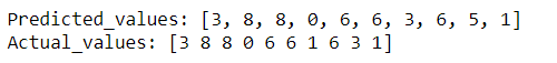
Comparing the predicted value to the Actual values to see how correct is model performing. In the below figure we can see the difference in the Predicted VS Actual values.
y_classes = [np.argmax(element) for element in pred]
print('Predicted_values:',y_classes[:10])
print('Actual_values:',y_test[:10])
As we saw that our model was overfitting, we can improve your model performance and decrease the overfitting using some additional steps such as adding Dropouts to the model or performing Data Augmentation as the overfitting problem can also be due to less amount of data available.
Here, I will show how we can use Dropouts for reducing overfitting. I’ll be defining a new model for the same.
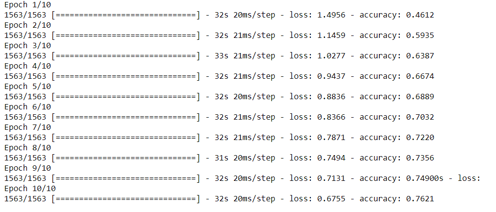
model4=Sequential()
#adding the first Convolution layer
model4.add(Conv2D(32,(3,3),activation='relu',input_shape=(32,32,3)))
#adding Max pooling layer
model4.add(MaxPool2D(2,2))
#adding dropout
model4.add(Dropout(0.2))
#adding another Convolution layer
model4.add(Conv2D(64,(3,3),activation='relu'))
model4.add(MaxPool2D(2,2))
#adding dropout
model4.add(Dropout(0.2))
model4.add(Flatten())
#adding dense layer
model4.add(Dense(216,activation='relu'))
#adding dropout
model4.add(Dropout(0.2))
#adding output layer
model4.add(Dense(10,activation='softmax'))
model4.compile(optimizer='adam',loss='sparse_categorical_crossentropy',metrics=['accuracy'])
model4.fit(X_train,y_train,epochs=10)
model4.evaluate(X_test,y_test)

By this model, we have got a training accuracy of 76%(which is less than the first model) but we have got the test accuracy of 72% which means the problem of overfitting has been resolved to some extent.
Endnotes:
That’s how we implement CNN in Python. The dataset used here is a simple one and can be used for learning purposes but make sure to implement CNN on larger and complex datasets as well. That will help to discover more challenges and solutions as well. In future blogs, I will come up with some interesting and complex problems to solve using CNN.
About the Author
I am Deepanshi Dhingra currently working as a Data Science Researcher, and possess knowledge of Analytics, Exploratory Data Analysis, Machine Learning, and Deep Learning. Feel free to content with me on LinkedIn for any feedback and suggestions.


