Ensemble Stacking for Machine Learning and Deep Learning
Introduction
In this blog, we’ll be discussing Ensemble Stacking through theory and hands-on code!
Let’s begin with discussing what are Ensemble techniques?
Ensemble techniques are the methods that use multiple learning algorithms or models to produce one optimal predictive model. The model produced has better performance than the base learners taken alone. Other applications of ensemble learning also include selecting the important features, data fusion, etc. Ensemble techniques can be primarily classified into Bagging, Boosting, and Stacking.
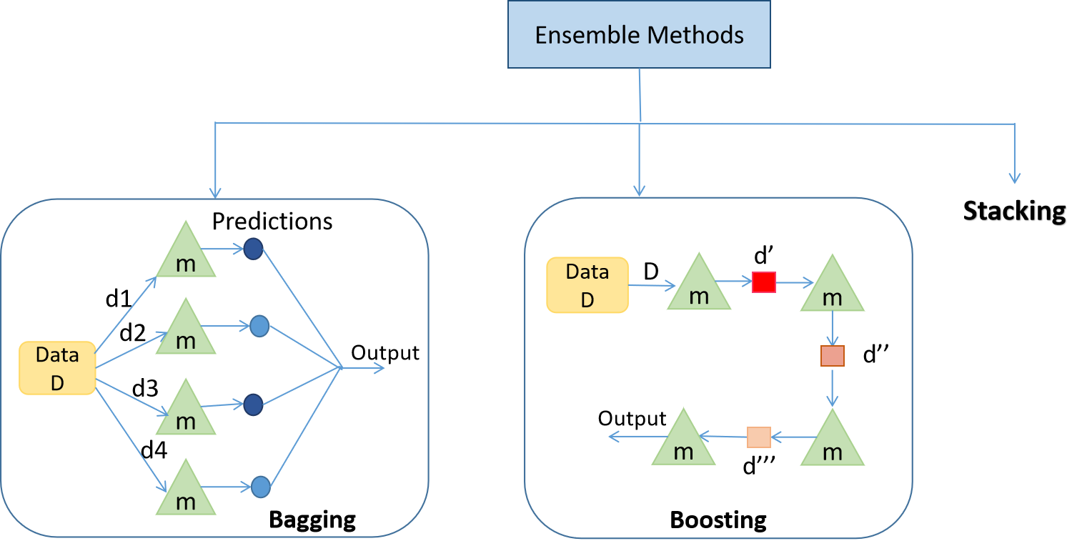
1. Bagging: Bagging is mainly applied in supervised learning problems. It involves two steps, i.e., bootstrapping and aggregation. Bootstrapping is a random sampling method in which samples are derived from the data using the replacement procedure. In Fig 1., the first step in bagging is bootstrapping, where random data samples are fed to each base learner. The base learning algorithm is run on the samples to complete the procedure. In Aggregation, the outputs from the base learners are combined. The goal is to increase the accuracy meanwhile reducing variance to a large extent. Eg.- RandomForest where the predictions from decision trees(base learners) are taken parallelly. In the case of regression problems, these predictions are averaged to give the final prediction and in the case of classification problems, the mode is selected as the predicted class.
2. Boosting: It is an ensemble method in which each predictor learns from preceding predictor mistakes to make better predictions in the future. The technique combines several weak base learners that are arranged in a sequential (Fig 1.) manner such that weak learners learn from the previous weak learner’s errors to create a better predictive model. Hence one strong learner is formed through significantly improving the predictability of models. Eg. – XGBoost, AdaBoost.
Now since we have discussed ensembling and the 2 types of ensemble methods, it’s the time we discuss Stacking!
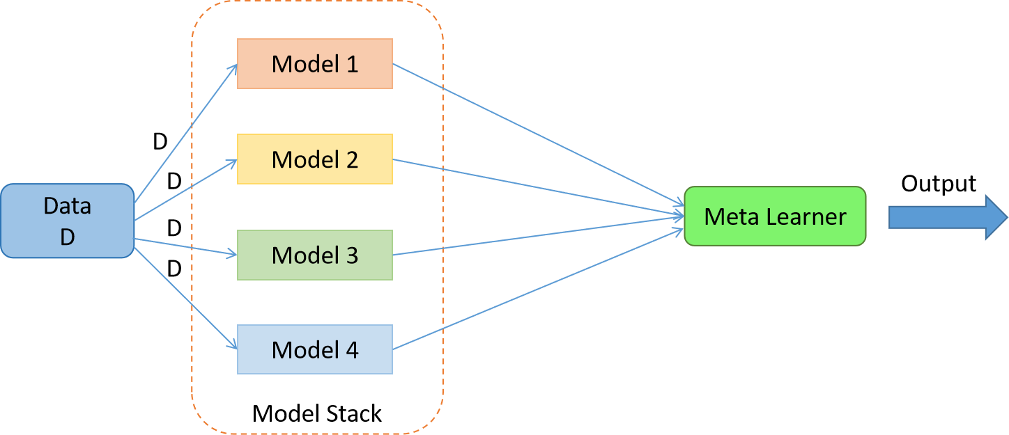
3. Stacking: While bagging and boosting used homogenous weak learners for ensemble, Stacking often considers heterogeneous weak learners, learns them in parallel, and combines them by training a meta-learner to output a prediction based on the different weak learner’s predictions. A meta learner inputs the predictions as the features and the target being the ground truth values in data D(Fig 2.), it attempts to learn how to best combine the input predictions to make a better output prediction.
In averaging ensemble eg. Random Forest, the model combines the predictions from multiple trained models. A limitation of this approach is that each model contributes the same amount to the ensemble prediction, irrespective of how well the model performed. An alternate approach is a weighted average ensemble, which weighs the contribution of each ensemble member by the trust on their contribution in giving the best predictions. The weighted average ensemble provides an improvement over the model average ensemble.
A further generalization of this approach is replacing the linear weighted sum with Linear Regression (regression problem) or Logistic Regression (classification problem) to combine the predictions of the sub-models with any learning algorithm. This approach is called Stacking.
In stacking, an algorithm takes the outputs of sub-models as input and attempts to learn how to best combine the input predictions to make a better output prediction.
Enough of the theory. Let’s see the hands-on part!
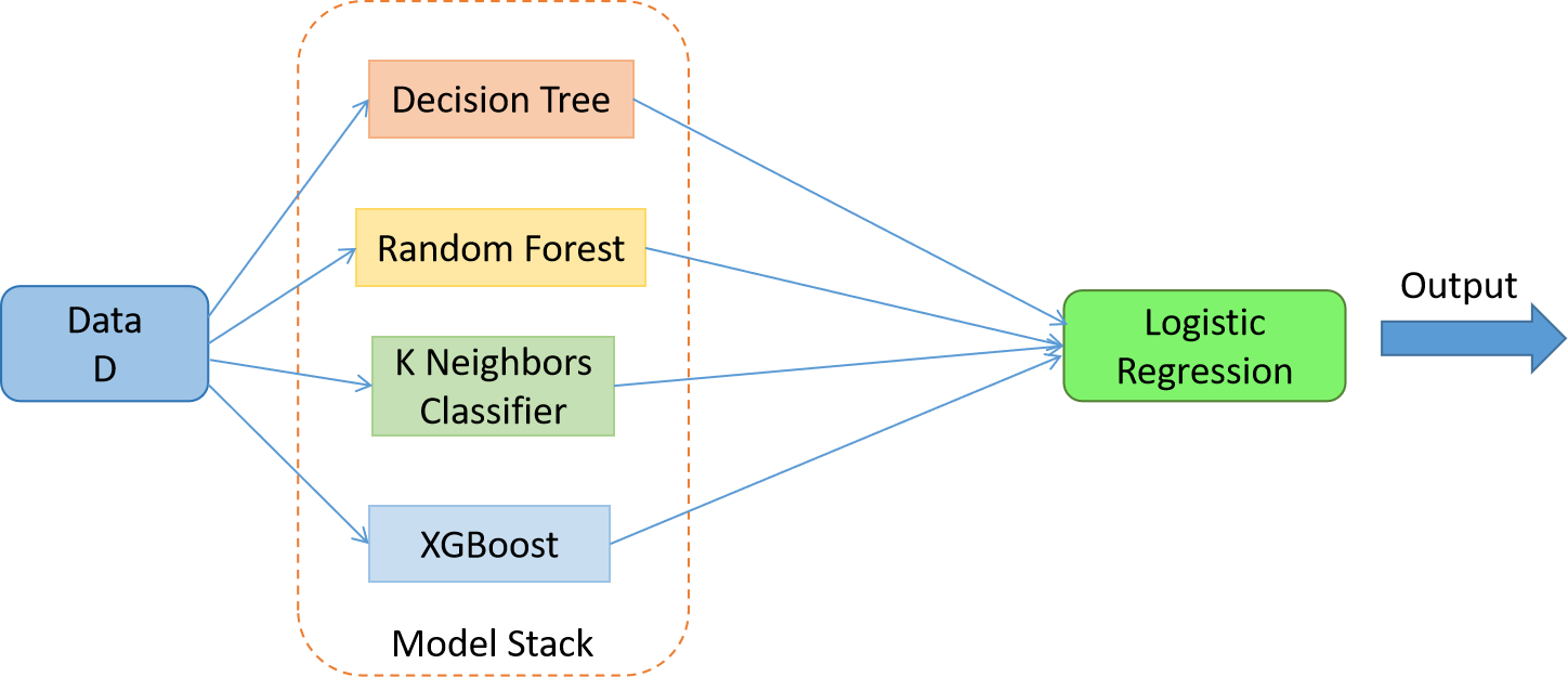
Stacking for Machine Learning
Dataset – Sklearn Breast Cancer Dataset (Classification)
Note – The data preprocessing part isn’t included in the following code. Kindly go through the link for the full code.
Load the base learning algorithms that you want to stack –
dtc =  DecisionTreeClassifier()
rfc = RandomForestClassifier()
knn =  KNeighborsClassifier()
xgb = xgboost.XGBClassifier()
Perform cross-validation and record the scores –
clf = [dtc,rfc,knn,xgb]
for algo in clf:
    score = cross_val_score( algo,X,y,cv = 5,scoring = 'accuracy')
    print("The accuracy score of {} is:".format(algo),score.mean())
Perform stacking and cross-validation –
dtc =  DecisionTreeClassifier()
rfc = RandomForestClassifier()
knn =  KNeighborsClassifier()
xgb = xgboost.XGBClassifier()
clf = [('dtc',dtc),('rfc',rfc),('knn',knn),('xgb',xgb)] #list of (str, estimator)
from sklearn.ensemble import StackingClassifier
lr = LogisticRegression()
stack_model = StackingClassifier( estimators = clf,final_estimator = lr)
score = cross_val_score(stack_model,X,y,cv = 5,scoring = 'accuracy')
print("The accuracy score of is:",score.mean())
The stacked model gives an accuracy score of 0.969 higher than any other base learning algorithm taken alone!
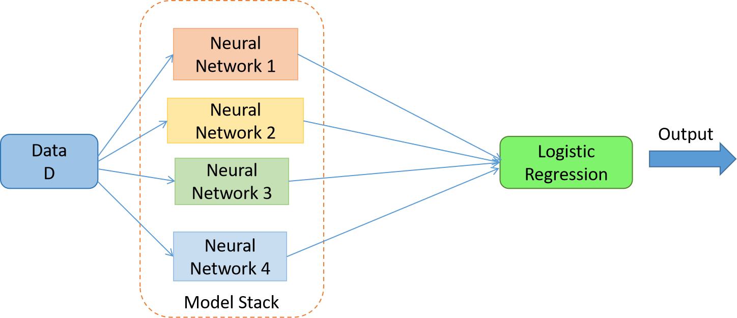
Stacking for Deep Learning
Dataset – Churn Modeling Dataset. Please go through the dataset for a better understanding of the below code.
Note – 1. The data preprocessing part isn’t included in the following code. Kindly go through the link for the full code; 2. Keras doesn’t provide a function to create a stack of deep neural networks. So we create a function of our own; 3. The Churn Modeling dataset has 10000 examples (rows). I split the data into training and testing with a ratio of 70:30.
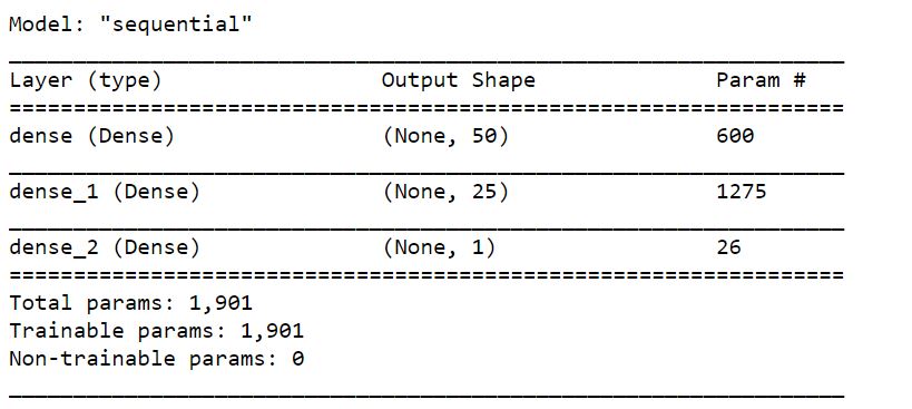
Create neural network architecture –
model1 = Sequential()
model1.add(Dense(50,activation = 'relu',input_dim = 11))
model1.add(Dense(25,activation = 'relu'))
model1.add(Dense(1,activation = 'sigmoid'))
I chose the loss function as binary cross-entropy, optimizer as adam, and F1-score as the error metric. Since F1-score isn’t available in Keras, we build of our own –
def recall_m(y_true, y_pred):
    true_positives = K.sum(K.round(K.clip(y_true * y_pred, 0, 1)))
    possible_positives = K.sum(K.round(K.clip(y_true, 0, 1)))
    recall = true_positives / (possible_positives + K.epsilon())
    return recall

def precision_m(y_true, y_pred):
    true_positives = K.sum(K.round(K.clip(y_true * y_pred, 0, 1)))
    predicted_positives = K.sum(K.round(K.clip(y_pred, 0, 1)))
    precision = true_positives / (predicted_positives + K.epsilon())
    return precision

def f1_m(y_true, y_pred):
    precision = precision_m(y_true, y_pred)
    recall = recall_m(y_true, y_pred)
    return 2*((precision*recall)/(precision+recall+K.epsilon()))
Train the model and record the performance. I chose epochs = 100 –
model1.compile(loss='binary_crossentropy', optimizer='adam', metrics=[f1_m])
history = model1.fit(X_train,y_train,validation_data = (X_test,y_test),epochs = 100)
Create 3 different neural network architectures and train them with the same settings –
model2 = Sequential()
model2.add(Dense(25,activation = 'relu',input_dim = 11))
model2.add(Dense(25,activation = 'relu'))
model2.add(Dense(10,activation = 'relu'))
model2.add(Dense(1,activation = 'sigmoid'))
model2.compile(loss='binary_crossentropy', optimizer='adam', metrics=[f1_m])
history1 = model2.fit(X_train,y_train,validation_data = (X_test,y_test),epochs = 100)
model3 = Sequential()
model3.add(Dense(50,activation = 'relu',input_dim = 11))
model3.add(Dense(25,activation = 'relu'))
model3.add(Dense(25,activation = 'relu'))
model3.add(Dropout(0.1))
model3.add(Dense(10,activation = 'relu'))
model3.add(Dense(1,activation = 'sigmoid'))
model3.compile(loss='binary_crossentropy', optimizer='adam', metrics=[f1_m])
history3 = model3.fit(X_train,y_train,validation_data = (X_test,y_test),epochs = 100)
model4 = Sequential()
model4.add(Dense(50,activation = 'relu',input_dim = 11))
model4.add(Dense(25,activation = 'relu'))
model4.add(Dropout(0.1))
model4.add(Dense(10,activation = 'relu'))
model4.add(Dense(1,activation = 'sigmoid'))
model4.compile(loss='binary_crossentropy', optimizer='adam', metrics=[f1_m])
history4 = model4.fit(X_train,y_train,validation_data = (X_test,y_test),epochs = 100)
Save the models –
model1.save('model1.h5')
model2.save('model2.h5')
model3.save('model3.h5')
model4.save('model4.h5')
Load the models –
dependencies = {'f1_m': f1_m }
# create a custom function to load model
def load_all_models(n_models):
	all_models = list()
	for i in range(n_models):
		# Specify the filename
		filename = '/content/model' + str(i + 1) + '.h5'
		# load the model
		model = load_model(filename,custom_objects=dependencies)
		# Add a list of all the weaker learners
		all_models.append(model)
		print('>loaded %s' % filename)
	return all_models
n_members = 4
members = load_all_models(n_members)
print('Loaded %d models' % len(members))
Perform stacking –
We train the meta learner first by providing examples from the test set to the weak learners i.e the 4 neural networks and collecting the predictions. In this case, each model will output one prediction (‘exited’: 1 or ‘not exited’: 0) for each example. PS. Please go through the dataset. Therefore, the 3,000 examples in the test set will result in four arrays (since there 4 neural networks) with the shape [3000, 1].
We then combine these arrays into a three-dimensional array with the shape [3000, 4, 1] through dstack() NumPy function that will stack each new set of predictions.
As input for a new model, we will require 3,000 examples with some number of features. Given that we have four models and each model makes 1 prediction in each example, then we would have 4 (1 x 4) features for each example provided to the submodels. We can transform the [3000, 4, 1] shaped predictions from the sub-models into a [3000, 4] shaped array to be used to train a meta-learner using the reshape() NumPy function and flattening the final two dimensions. The stacked_dataset() function implements this step.
# create stacked model input dataset as outputs from the ensemble
def stacked_dataset(members, inputX):
	stackX = None
	for model in members:
		# make prediction
		yhat = model.predict(inputX, verbose=0)
		# stack predictions into [rows, members, probabilities]
		if stackX is None:
			stackX = yhat #
		else:
			stackX = dstack((stackX, yhat))
	# flatten predictions to [rows, members x probabilities]
	stackX = stackX.reshape((stackX.shape[0], stackX.shape[1]*stackX.shape[2]))
	return stackX
We have created the dataset to train the meta-learner. We fit the meta-learner on the data for training.
# fit a model based on the outputs from the ensemble members
def fit_stacked_model(members, inputX, inputy):
	# create dataset using ensemble
	stackedX = stacked_dataset(members, inputX)
	# fit the meta learner
	model = LogisticRegression() #meta learner
	model.fit(stackedX, inputy)
	return model
model = fit_stacked_model(members, X_test,y_test)
Make the predictions –
# make a prediction with the stacked model
def stacked_prediction(members, model, inputX):
	# create dataset using ensemble
	stackedX = stacked_dataset(members, inputX)
	# make a prediction
	yhat = model.predict(stackedX)
	return yhat
# evaluate model on test set -
yhat = stacked_prediction(members, model, X_test)
score = f1_m(y_test/1.0, yhat/1.0)
print('Stacked F Score:', score)
The stacked model gives an F-score of 0.6007 on test data which is higher than any other neural network taken alone!
With this, we can conclude that the stacked model can give better performance than the individual models. No doubt why Stacking Ensembling is the favorite approach to win hackathons and give state-of-the-art results.
Do check the Github repo for the codes and the respective outputs.
With this, we come to the end of the blog. I hope the blog was informative. Feedback for the blog is most welcomed. Happy Learning 🙂
About the author
I am Yash Khandelwal, an undergrad at BIT Mesra. I am pursuing an Integrated MSc in Mathematics and Computing. Feel free to connect with me!
Connect with me on Linked in – https://www.linkedin.com/in/yash-khandelwal-a40484bb/
Follow me on Github – https://github.com/YashK07


Informative article thank you. Query: Is this possible for the stacked model with meta learner = a deep learning-based model and weak learners = 4 machine learning-based models? Can you please guide me with the implementation?