Training BERT Text Classifier on Tensor Processing Unit (TPU)

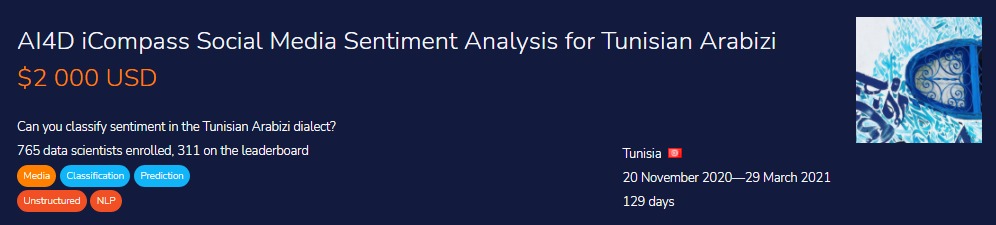
Training hugging face most famous model on TPU for social media Tunisian Arabizi sentiment analysis.

Introduction

The Arabic speakers usually express themself in local dialect on social media, so Tunisians use Tunisian Arabizi which consists of Arabic written in form of Latin alphabets. The sentiment analysis relies on cultural knowledge and word sense with contextual information. We will be using both Arabizi dialect and sentimental analysis to solve the problem in this project.

The competition is hosted on Zindi which is organized by AI4D. In this competition, we are provided with train and test datasets. The train data set consists of Arabizi text with the sentiment of that text. We need to build a model and improve our metric to score the top position in the competition leader board.

The dataset was collected from different social media platforms and the objective of this project is to predict labels of the test dataset. The label will determine whether our sentence has positive, negative, or neutral sentiments AI4D iCompass.

Description

In this project, we will be training the multilingual BERT model using TPU.

TPU

Tensor Processing Unit (TPU) is an Artificial Intelligence accelerator application-specific integrated circuit (ASIC) developed by Google which helps reduce training time on deep learning models especially Google’s own TensorFlow package Tensor Processing Unit. Training your deep learning model on TPU is much simpler in the TensorFlow python library as compared to PyTorch.

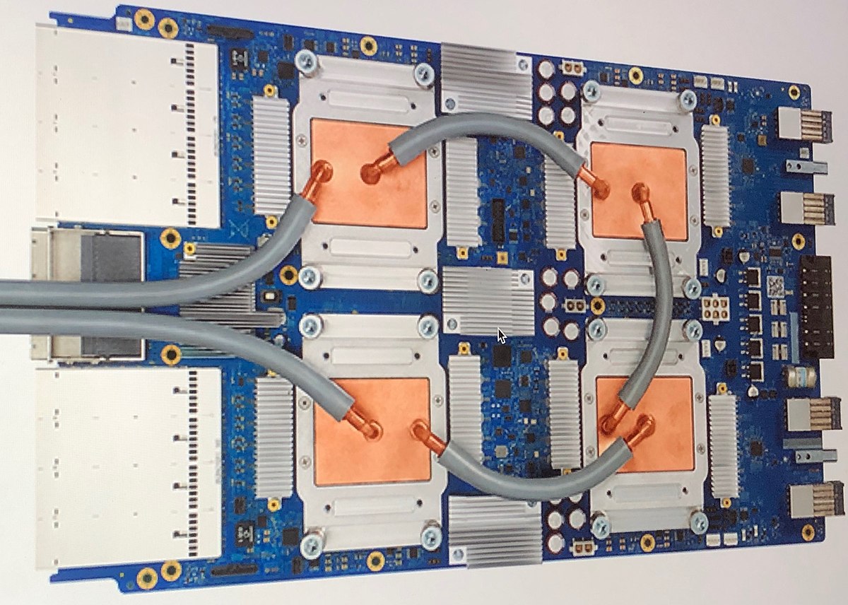
The cloud TPUs resources minimize time to compute linear algebra problems and machine learning applications are developed using most linear algebras. Previously, it took weeks to train a complex deep learning model with huge data set but using TPUs the train time is reduced to few hours. Google Cloud.

BERT

BERT (Bidirectional Encoder Representations from Transformers) is an NLP (Natural Language Processing Model) proposed by researchers at Google Research in 2018. BERT is basically an Encoder stack of transformer architecture analyticsvidhya. Initially, when BERT has released it over, took other models in terms of accuracy on many NLP tasks and soon after other researcher started using BERT architecture and releasing newer and better models’ versions in different languages. This is where our BERT base multilingual cased model comes, which performed quite well on new low resource language. Our model was pretrained on the top 104 languages using the largest Wikipedia corpus of multilingual data and to learn more on this model read the paper. The researchers used masked language modeling (MLM) to make it effective for multiple languages. To find more on the model please check model card bert-base-multilingual-cased.

Code

We will start with setting up our model to train on TPU and then we will set our hyperparameters to improve the performance. We will be loading and training Tunisian Arabizi dialect sentimental analysis data and then predicting on the test data set provided by ai4d.ai.

Import Libraries

We have imported all necessary libraries for us to experiment on or pretrained the BERT model.

import tensorflow as tf
import logging
from tensorflow.keras.layers import (
    Dense,
    Flatten,
    Conv1D,
    Dropout,
    Input,
)
from tensorflow.keras.models import Sequential
from tensorflow.keras.optimizers import Adam
from tensorflow.keras import Model
from tensorflow.keras import regularizers
from transformers import BertTokenizer, TFBertModel
import os
import pandas as pd
import numpy as np
from sklearn.model_selection import train_test_split
from tqdm import tqdm
tqdm.pandas()
import re
import random

Setting up for TPU

The code is trying to check the TPU cluster, then initialize the TPU, and finally creating a TPU strategy which we will use later to train our model on Cloud. If you don’t have TPU the code will shift to either GPU or CPU depending on your machine.

try:
    tpu = tf.distribute.cluster_resolver.TPUClusterResolver()
    tf.config.experimental_connect_to_cluster(tpu)
    tf.tpu.experimental.initialize_tpu_system(tpu)
    strategy = tf.distribute.experimental.TPUStrategy(tpu)
except ValueError:
    strategy = tf.distribute.get_strategy() # for CPU and single GPU
    print('Number of replicas:', strategy.num_replicas_in_sync)

Setting up hyperparameters

These hyperparameters are for experimentations so that we can make changes and get better results. For now, these parameter produces best results so far.

max_length = 140
batch_size = 16
dev_size = 0.1
num_class = 4

Loading BERT Tokenizer

Downloading BERT tokenizer from Hugging face using transformers library.

model_name = "bert-base-multilingual-cased"
tokenizer = BertTokenizer.from_pretrained(model_name)

Downloading: 100% 996k/996k [00:00<00:00, 5.62MB/s]

Downloading: 100% 29.0/29.0 [00:00<00:00, 950B/s]

Downloading: 100% 1.96M/1.96M [00:00<00:00, 11.8MB/s]

Reading train dataset

Train dataset contains 70,000 samples whereas our test dataset contains 30,000 samples. The train data set have an id column that contains a unique identifier, text columns that contain tweets written in Arabizi dialect, and a label column that contains sentiments {-1,0,1}.

• Reading Data: Used pandas to read CSV file
• Dropping duplicate tweets: This improves the performance of the model  
• Remapping labels: This made it easy to encode and decode -1 sentiment and eventually improved our performance metric.
• train dev split: for training and evaluation.

train_df = pd.read_csv('../input/aranizi-dailect-training-data/Arabizi-Dailect-Train.csv')

train_df.text = train_df.text.astype(str)
train_df.drop_duplicates(subset=['text'],inplace=True)
train_df.label=train_df.label.map({-1:0,1:2,0:1})
train, dev = train_test_split(train_df, test_size=dev_size, random_state=42)

Loading data and processing it

We are using transformers batch encode plus to encode out text data and limiting the max length to 150. We have used the TensorFlow function to convert our labels into the categorical type and loaded them into a TensorFlow dataset which prepares our data to be used by the model. I thought cache helps TPU to store data, but you can either remove it or add it, your model will work in any case.

def bert_encode(data):
    tokens = tokenizer.batch_encode_plus(
        data, max_length=max_length, padding="max_length", truncation=True
    )
    return tf.constant(tokens["input_ids"])
train_encoded = bert_encode(train.text)
dev_encoded = bert_encode(dev.text)
train_labels = tf.keras.utils.to_categorical(train.label.values, num_classes=num_class)
dev_labels = tf.keras.utils.to_categorical(dev.label.values, num_classes=num_class)
train_dataset = (
    tf.data.Dataset.from_tensor_slices((train_encoded, train_labels))
    .shuffle(100)
    .batch(batch_size)
).cache()
dev_dataset = (
    tf.data.Dataset.from_tensor_slices((dev_encoded, dev_labels))
    .shuffle(100)
    .batch(batch_size)
).cache()

Model

The model is influenced by lmasca‘s notebook available on Kaggle, he has used LSTM and I am just using the Dense layer with dropouts. Kaggle also provides 30 hours of free TPU which makes it easier for anyone to use cloud computing for free.

Our model is quite simple, we have used the same BERT architecture and added 3 Dense layers with a dropout rate = 0.3. I am using relu activation from the first two layers and for the output layer, we have used soft plus which performed amazingly on TPU.

I have also experimented with Bidirectional Dense LSTM layers and simple LSTM, but those model didn’t perform well. 

def bert_tweets_model():
    bert_encoder = TFBertModel.from_pretrained(model_name, output_attentions=True)
    input_word_ids = Input(
        shape=(max_length,), dtype=tf.int32, name="input_ids"
    )
    last_hidden_states = bert_encoder(input_word_ids)[0]
    clf_output = Flatten()(last_hidden_states)
    net = Dense(512, activation="relu")(clf_output)
    net = Dropout(0.3)(net)
    net = Dense(440, activation="relu")(net)
    net = Dropout(0.3)(net)
    output = Dense(num_class, activation="softplus")(net)
    model = Model(inputs=input_word_ids, outputs=output)
    return model

Compiling Model

You need to add with strategy.scope(): and run our model which will download the model from the HuggingFace server and load it into a model variable. Your model, optimizer, and model compilation should be done under strategy.scope() to properly train on Cloud TPU.

with strategy.scope():
    model = bert_tweets_model()
    adam_optimizer = Adam(learning_rate=1e-5)
    model.compile(
        loss="categorical_crossentropy", optimizer=adam_optimizer, metrics=["accuracy"]
    )
    model.summary()

Downloading: 100% 625/625 [00:00<00:00, 19.9kB/s]

Downloading: 100% 1.08G/1.08G [00:38<00:00, 29.6MB/s]

Model Structure

You can see the model structure and the Dense layers we added with Dropout.

Model: "model_1"
_________________________________________________________________
Layer (type)                 Output Shape              Param #   
=================================================================
input_ids (InputLayer)       [(None, 140)]             0         
_________________________________________________________________
tf_bert_model_1 (TFBertModel TFBaseModelOutputWithPool 177853440 
_________________________________________________________________
flatten_1 (Flatten)          (None, 107520)            0         
_________________________________________________________________
dense_3 (Dense)              (None, 512)               55050752  
_________________________________________________________________
dropout_76 (Dropout)         (None, 512)               0         
_________________________________________________________________
dense_4 (Dense)              (None, 440)               225720    
_________________________________________________________________
dropout_77 (Dropout)         (None, 440)               0         
_________________________________________________________________
dense_5 (Dense)              (None, 4)                 1764      
=================================================================
Total params: 233,131,676
Trainable params: 233,131,676
Non-trainable params: 0
_________________________________________________________________

Training Model

It’s finally time for us to train our model on TPU. The model took 17 minutes to train on TPU, 45 minutes to train on GPU, and 2.5 hours to train on CPU. You can see the performance difference clearly. By using model.fit we have trained our model on the training dataset and used dev_dataset as validation. Our train accuracy improved with each epoch as well as our validation accuracy.

history = model.fit(
    train_dataset,
    batch_size=batch_size,
    epochs=5,
    validation_data=dev_dataset,
    verbose=1,
)

Epoch 1/5
4166/4166 [==============================] - 313s 60ms/step - loss: 0.7691 - accuracy: 0.6309 - val_loss: 0.4994 - val_accuracy: 0.7810
Epoch 2/5
4166/4166 [==============================] - 246s 59ms/step - loss: 0.5092 - accuracy: 0.7870 - val_loss: 0.4541 - val_accuracy: 0.8027
Epoch 3/5
4166/4166 [==============================] - 248s 59ms/step - loss: 0.4232 - accuracy: 0.8271 - val_loss: 0.4680 - val_accuracy: 0.8081
Epoch 4/5
4166/4166 [==============================] - 247s 59ms/step - loss: 0.3577 - accuracy: 0.8606 - val_loss: 0.4994 - val_accuracy: 0.8103
Epoch 5/5
4166/4166 [==============================] - 247s 59ms/step - loss: 0.2980 - accuracy: 0.8849 - val_loss: 0.6219 - val_accuracy: 0.8166

Saving Weights

Let’s save or model so that we can use it again or deploy it as streamlit web app.

model.save_weights('weights.h5', overwrite=True)

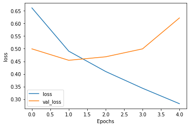
Display Loss and Accuracy

We can see the results in the line plot below with every epoch our training and validation accuracy improved. The story in the loss line plot is quite different, after epoch 3 the loss started to increase. We should keep the number of epoch to 3 to get better results on the test dataset.

import matplotlib.pyplot as plt
def plot_graphs(history, string):
    plt.plot(history.history[string])
    plt.plot(history.history["val_" + string])
    plt.xlabel("Epochs")
    plt.ylabel(string)
    plt.legend([string, "val_" + string])
    plt.show()
plot_graphs(history, "accuracy")
plot_graphs(history, "loss")

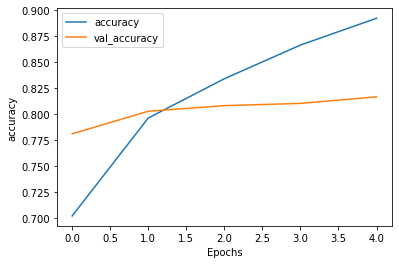
Image by Author | Accuracy lineplot