Building Resnet-34 model using Pytorch – A Guide for Beginners
This article was published as a part of the Data Science Blogathon
Introduction
Deep learning has evolved a lot in recent years and we all are excited to build deeper architecture networks to gain more accuracies for our models. These techniques are widely tried for Image related works like classification, clustering, or synthesis. Going deep may look cool but won’t help as neural networks face an issue called degradation.
The accuracy is affected to a great extent here. This also leads to a problem called Vanishing gradient descend. This won’t allow us to properly update the weights during the backpropagation step. During the backpropagating step, we use the chain rule, the derivatives of each layer as we go down the network get multiplied.
If we use deeper layers and have hidden layers like sigmoid, the derivatives are scaled-down below 0.25 within each layer. So when a lot of layers derivatives get multiplied the gradient decreases exponentially and we get a very small value which is useless for the gradient calculation. This lead to the making of Resnet by Microsoft Research which used skipped connections to avoid degradation. In this article, we will discuss an implementation of 34 layered ResNet architecture using the Pytorch framework in Python.
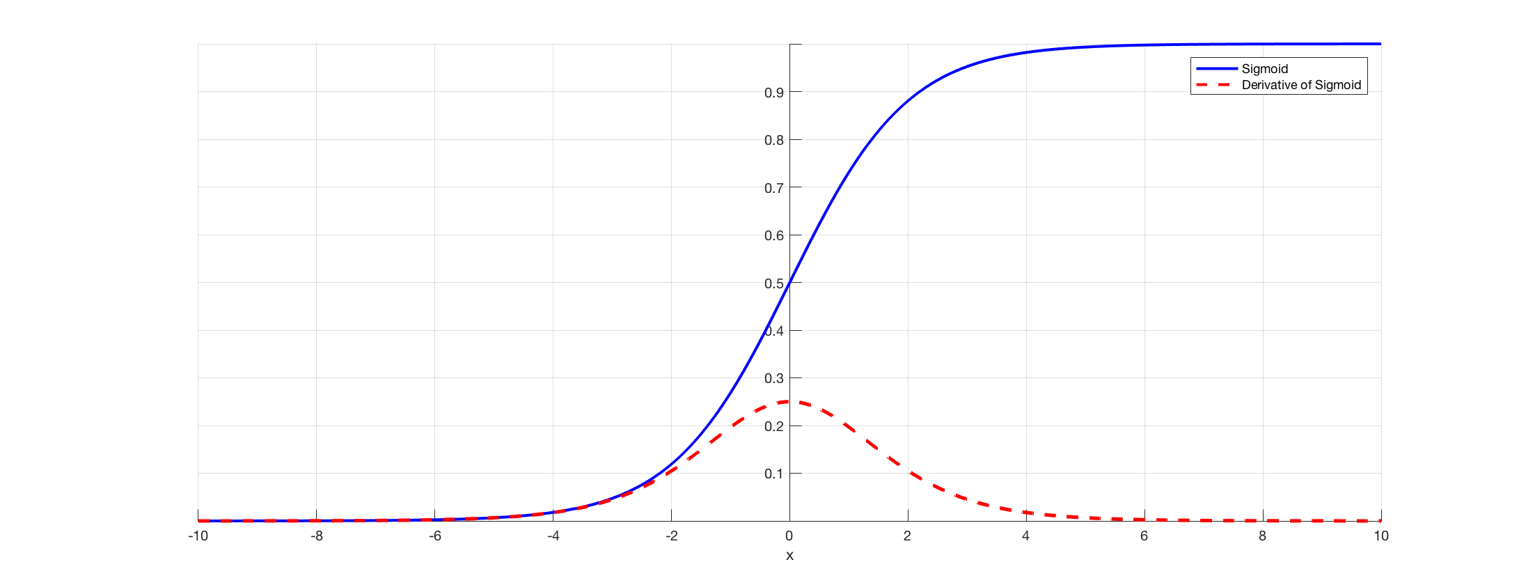
As discussed above this diagram shows us the vanishing gradient problem. The derivatives of sigmoid functions are scaled-down below 0.25 and this losses lot of information while updating the gradients.
The issue with plane networks
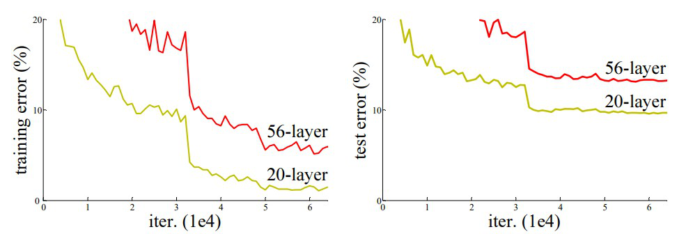
As shown in the figure, we see the plane networks, that have deeper layers. On the left, we have train error and test error on the right. We would be thinking that this could be a sue to overfitting, but here the error% of the 56-layer network is much worst on both training as well as the testing data which does not happen when the model is overfitting. This is called degradation.
Architecture of Resnet-34
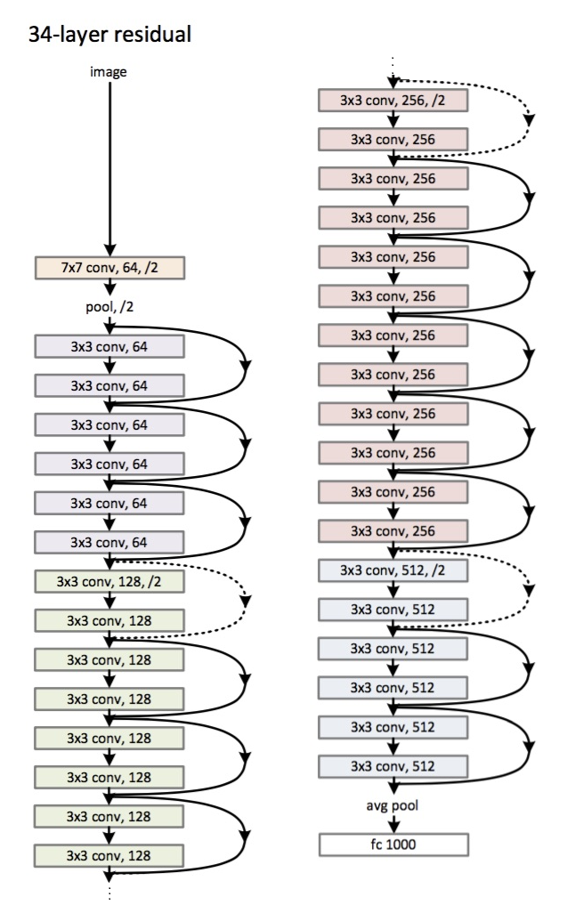
Initially, we have a convolutional layer that has 64 filters with a kernel size of 7×7 this is the first convolution, then followed by a max-pooling layer. We have the stride specified as 2 in both cases. Next, in conv2_x we have the pooling layer and the following convolution layers. These layers are normally grouped in pairs because of the way the residuals are connected (the arrows show that are jumping every two layers).
Here, we have the 2 layers of which have a kernel_sizeof 3×3, num_filters of 64, and all these are repeated x3, which corresponds to the layers between the pool,/2 and the filter 128 ones, 6 layers in total (one pair times 3). These 2 layers are kernel_size of 3×3, num_filters is 128, and these are also get repeated but on this times 4. This continues until the avg_pooling and the softmax function. Each time the number of filters gets doubled we can see the first layer specifies num_filters/2.
Code for defining Resnet-34 in Pytorch:
class ResNet34(nn.Module):
    def __init__(self):
        super(ResNet34,self).__init__()

        self.block1 = nn.Sequential(
            nn.Conv2d(1,64,kernel_size=2,stride=2,padding=3,bias=False),
            nn.BatchNorm2d(64),
            nn.ReLU(True)
        )

        self.block2 = nn.Sequential(
            nn.MaxPool2d(1,1),
            ResidualBlock(64,64),
            ResidualBlock(64,64,2)
        )

        self.block3 = nn.Sequential(
            ResidualBlock(64,128),
            ResidualBlock(128,128,2)
        )

        self.block4 = nn.Sequential(
            ResidualBlock(128,256),
            ResidualBlock(256,256,2)
        )
        self.block5 = nn.Sequential(
            ResidualBlock(256,512),
            ResidualBlock(512,512,2)
        )

        self.avgpool = nn.AvgPool2d(2)
        # vowel_diacritic
        self.fc1 = nn.Linear(512,11)
        # grapheme_root
        self.fc2 = nn.Linear(512,168)
        # consonant_diacritic
        self.fc3 = nn.Linear(512,7)

    def forward(self,x):
        x = self.block1(x)
        x = self.block2(x)
        x = self.block3(x)
        x = self.block4(x)
        x = self.block5(x)
        x = self.avgpool(x)
        x = x.view(x.size(0),-1)
        x1 = self.fc1(x)
        x2 = self.fc2(x)
        x3 = self.fc3(x)
        return x1,x2,x3
This code gives us complete implementation of a module for Resnet-34. Now let’s dive deep into understanding how each line works. For this let’s shorten the architecture we saw earlier. Refer to the 34 layered diagrams below.

We can see that we need to implement any Resnet architecture in 5 blocks. The first block has 64 filters with a stride of 2. followed by max-pooling with stride 2. The architecture uses padding of 3. Since there is a chance of internal covariate shift we must stabilize the network by batch normalization. We use ReLU activation at the end. The first block is the same for any architecture and the rest blocks are changed for different layers and are repeated in a specific pattern. 1st block can be implemented as:
nn.Conv2d(1,64,kernel_size=2,stride=2,padding=3,bias=False),
nn.BatchNorm2d(64),
nn.ReLU(True)
At this point, we have a skip connection. Which is the main idea of residual networks. The architecture diagram we saw earlier had skipped connections show with dotted and dark arrows. The dotted line is what’s happening here as we are moving into a channel with more size than the earlier one. The second block has the implementation of an initial max pool of 1 * 1 with a kernel size of 3 * 3 and two residual blocks as shown in the code below. These two take in 64 as input and output channels and are repeated 3 times as shown in architecture. In the end, the last one is connected to the next block with a stride of 2.
nn.MaxPool2d(1,1),
ResidualBlock(64,64),
ResidualBlock(64,64,2)
The last block’s content got repeated 3 times and we had indicated that with the dark arrow in the architecture diagram and the input and output channel size remains the same. The ‘/2’ shown in the architecture diagram tells us about the stride used.
The third block takes a kernel size of 3 * 3 with an input channel coming from the last block of 64 and giving an output channel of 128. Then we take the same 128 as input and 128 as output channel. We repeat this 4 times as shown in the earlier architecture diagram.
ResidualBlock(64,128),
ResidualBlock(128,128,2)
Similarly to this, we build our 4rth and 5th blocks that have 256 and 512 as kernel sizes.
ResidualBlock(128,256),
ResidualBlock(256,256,2)
ResidualBlock(256,512),
ResidualBlock(512,512,2)
The Linear functions help connect this finally with the end mission which may include steps like classifying the cifar 10 datasets, etc. and the idea is to flatten the layers and give a probabilistic value to find the max. And the forward function we defined to connect each of the blocks. For the complete python implementation including training, you may refer to this website. We can also make use of Pytorch’s transfer learning technique and for that code, you may refer to this GitHub repo.
Conclusion:
Reference:
- https://www.kaggle.com/khoongweihao/resnet-34-pytorch-starter-kit
- https://datascience.stackexchange.com/questions/33022/how-to-interpert-resnet50-layer-types
About Me: I am a Research Student interested in the field of Deep Learning and Natural Language Processing and currently pursuing post-graduation in Artificial Intelligence.
Image Source
- Image 1,2: https://towardsdatascience.com/the-vanishing-gradient-problem-69bf08b15484
- Image 3,4: https://datascience.stackexchange.com/questions/33022/how-to-interpert-resnet50-layer-types
- Preview Image: https://www.zdnet.com/pictures/10-cool-robots-at-this-years-robobusiness-conference/2/
Feel free to connect with me on:
- Linkedin: https://www.linkedin.com/in/siddharth-m-426a9614a/
- Github: https://github.com/Siddharth1698


