Deep Learning in the Trenches: Understanding Inception Network from Scratch

Introduction

Deep learning is rapidly gaining steam as more and more research papers emerge from around the world. These papers undoubtedly contain a ton of information, but they can often be difficult to parse through. And to understand them, you might have to go through that paper multiple number of times (and perhaps even other dependent papers!).

This is truly a daunting task for non-academicians like us.

Personally, I find the task of going through a research paper, interpreting the crux behind it, and implementing the code as an important skill every deep learning enthusiast and practitioner should possess. Practically implementing research ideas brings out the thought process of the author and also helps transform those ideas into real-world industry applications.

So in this article (and the subsequent series of articles) my motive of writing is two-fold:

1. Enable the readers to keep abreast with cutting edge research by breaking down deep learning papers into understandable concepts
2. Learn to convert research ideas to code myself, and encourage people to do so simultaneously

This article assumes that you have a good grasp on the basics of deep learning. In case you don’t, or simply need a refresher, check out the below articles first and then head back here pronto:

• Fundamentals of Deep Learning – Starting with Artificial Neural Network
• Tutorial: Optimizing Neural Networks using Keras

Summary of the “Going Deeper with Convolutions” Paper

This article focuses on the paper “Going deeper with convolutions” from which the hallmark idea of inception network came out. Inception network was once considered a state-of-the-art deep learning architecture (or model) for solving image recognition and detection problems.

It put forward a breakthrough performance on the ImageNet Visual Recognition Challenge (in 2014), which is a reputed platform for benchmarking image recognition and detection algorithms. Along with this, it set off a ton of research in the creation of new deep learning architectures with innovative and impactful ideas.

We will go through the main ideas and suggestions propounded in the aforementioned paper and try to grasp the techniques within. In the words of the author:

“In this paper, we will focus on an efficient deep neural network architecture for computer vision, code named Inception, which derives its name from (…) the famous “we need to go deeper” internet meme.”

That does sound intriguing, doesn’t it? Well, read on then!

Objective of the Paper

There’s a simple but powerful way of creating better deep learning models. You can just make a bigger model, either in terms of deepness, i.e., number of layers, or the number of neurons in each layer. But as you can imagine, this can often create complications:

• Bigger the model, more prone it is to overfitting. This is particularly noticeable when the training data is small
• Increasing the number of parameters means you need to increase your existing computational resources

A solution for this, as the paper suggests, is to move on to sparsely connected network architectures which will replace fully connected network architectures, especially inside convolutional layers. This idea can be conceptualized in the below images:

This paper proposes a new idea of creating deep architectures. This approach lets you maintain the “computational budget”, while increasing the depth and width of the network. Sounds too good to be true! This is how the conceptualized idea looks:

Let us look at the proposed architecture in a bit more detail.

Proposed Architectural Details

The paper proposes a new type of architecture – GoogLeNet or Inception v1. It is basically a convolutional neural network (CNN) which is 27 layers deep. Below is the model summary:

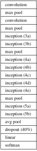
Notice in the above image that there is a layer called inception layer. This is actually the main idea behind the paper’s approach. The inception layer is the core concept of a sparsely connected architecture.

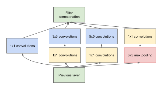
Let me explain in a bit more detail what an inception layer is all about. Taking an excerpt from the paper:

“(Inception Layer) is a combination of all those layers (namely, 1×1 Convolutional layer, 3×3 Convolutional layer, 5×5 Convolutional layer) with their output filter banks concatenated into a single output vector forming the input of the next stage.”

Along with the above-mentioned layers, there are two major add-ons in the original inception layer:

• 1×1 Convolutional layer before applying another layer, which is mainly used for dimensionality reduction
• A parallel Max Pooling layer, which provides another option to the inception layer

To understand the importance of the inception layer’s structure, the author calls on the Hebbian principle from human learning. This says that “neurons that fire together, wire together”. The author suggests that when creating a subsequent layer in a deep learning model, one should pay attention to the learnings of the previous layer.

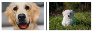
Suppose, for example, a layer in our deep learning model has learned to focus on individual parts of a face. The next layer of the network would probably focus on the overall face in the image to identify the different objects present there. Now to actually do this, the layer should have the appropriate filter sizes to detect different objects.

This is where the inception layer comes to the fore. It allows the internal layers to pick and choose which filter size will be relevant to learn the required information. So even if the size of the face in the image is different (as seen in the images below), the layer works accordingly to recognize the face. For the first image, it would probably take a higher filter size, while it’ll take a lower one for the second image.

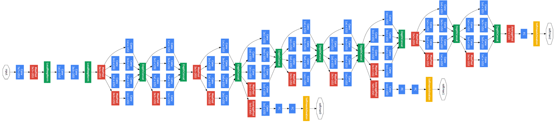
The overall architecture, with all the specifications, looks like this:

Training Methodology

Note that this architecture came about largely due to the authors participating in an image recognition and detection challenge. Hence there are quite a few “bells and whistles” which they have explained in the paper. These include:

• The hardware they used to train the models
• The data augmentation technique for creating the training dataset
• The hyperparameters of the neural network, like the optimization technique and the learning rate schedule
• Auxiliary training required for training the model
• Ensembling techniques they used to build the final submission

Among this, the auxiliary training done by the authors is quite interesting and novel in nature. So we will focus on that for now. The details for the rest of the techniques can be taken from the paper itself, or in the implementation which we will see below.

To prevent the middle part of the network from “dying out”, the authors introduced two auxiliary classifiers (the purple boxes in the image). They essentially applied softmax to the outputs of two of the inception modules, and computed an auxiliary loss over the same labels. The total loss function is a weighted sum of the auxiliary loss and the real loss. The weight value used in the paper was 0.3 for each auxiliary loss.

Implementation of GoogLeNet in Keras

Now that you have understood the architecture of GoogLeNet and the intuition behind it, it’s time to power up Python and implement our learnings using Keras! We will use the CIFAR-10 dataset for this purpose.

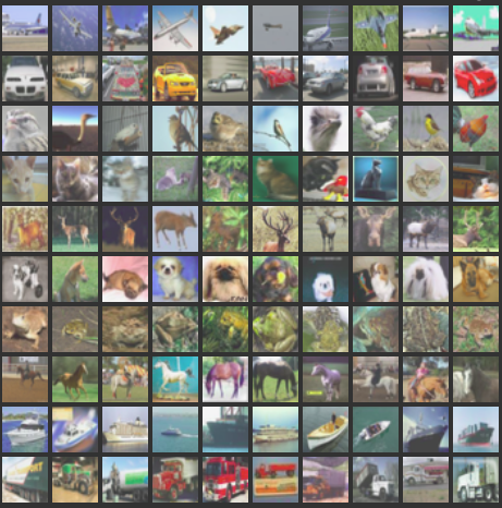
CIFAR-10 is a popular image classification dataset. It consists of 60,000 images of 10 classes (each class is represented as a row in the above image). The dataset is divided into 50,000 training images and 10,000 test images.

Note that you must have the required libraries installed to implement the code we will see in this section. This includes Keras and TensorFlow (as a back-end for Keras). You can refer to the official installation guide in case you don’t have Keras already installed on your machine.

Now that we have dealt with the prerequisites, we can finally start coding the theory we covered in the earlier sections. The first thing we need to do is import all the necessary libraries and modules which we will use throughout the code.

import keras
from keras.layers.core import Layer
import keras.backend as K
import tensorflow as tf
from keras.datasets import cifar10

import keras
from keras.layers.core import Layer
import keras.backend as K
import tensorflow as tf
from keras.datasets import cifar10

from keras.models import Model
from keras.layers import Conv2D, MaxPool2D,  \
    Dropout, Dense, Input, concatenate,      \
    GlobalAveragePooling2D, AveragePooling2D,\
    Flatten

import cv2 
import numpy as np 
from keras.datasets import cifar10 
from keras import backend as K 
from keras.utils import np_utils

import math 
from keras.optimizers import SGD 
from keras.callbacks import LearningRateScheduler

We will then load the dataset and perform some preprocessing steps. This is a critical task before the deep learning model is trained.

num_classes = 10

def load_cifar10_data(img_rows, img_cols):

    # Load cifar10 training and validation sets
    (X_train, Y_train), (X_valid, Y_valid) = cifar10.load_data()

    # Resize training images
    X_train = np.array([cv2.resize(img, (img_rows,img_cols)) for img in X_train[:,:,:,:]])
    X_valid = np.array([cv2.resize(img, (img_rows,img_cols)) for img in X_valid[:,:,:,:]])

    # Transform targets to keras compatible format
    Y_train = np_utils.to_categorical(Y_train, num_classes)
    Y_valid = np_utils.to_categorical(Y_valid, num_classes)
    
    X_train = X_train.astype('float32')
    X_valid = X_valid.astype('float32')

    # preprocess data
    X_train = X_train / 255.0
    X_valid = X_valid / 255.0

    return X_train, Y_train, X_valid, Y_valid

X_train, y_train, X_test, y_test = load_cifar10_data(224, 224)

Now, we will define our deep learning architecture. We will quickly define a function to do this, which, when given the necessary information, gives us back the entire inception layer.

def inception_module(x,
                     filters_1x1,
                     filters_3x3_reduce,
                     filters_3x3,
                     filters_5x5_reduce,
                     filters_5x5,
                     filters_pool_proj,
                     name=None):
    
    conv_1x1 = Conv2D(filters_1x1, (1, 1), padding='same', activation='relu', kernel_initializer=kernel_init, bias_initializer=bias_init)(x)
    
    conv_3x3 = Conv2D(filters_3x3_reduce, (1, 1), padding='same', activation='relu', kernel_initializer=kernel_init, bias_initializer=bias_init)(x)
    conv_3x3 = Conv2D(filters_3x3, (3, 3), padding='same', activation='relu', kernel_initializer=kernel_init, bias_initializer=bias_init)(conv_3x3)

    conv_5x5 = Conv2D(filters_5x5_reduce, (1, 1), padding='same', activation='relu', kernel_initializer=kernel_init, bias_initializer=bias_init)(x)
    conv_5x5 = Conv2D(filters_5x5, (5, 5), padding='same', activation='relu', kernel_initializer=kernel_init, bias_initializer=bias_init)(conv_5x5)

    pool_proj = MaxPool2D((3, 3), strides=(1, 1), padding='same')(x)
    pool_proj = Conv2D(filters_pool_proj, (1, 1), padding='same', activation='relu', kernel_initializer=kernel_init, bias_initializer=bias_init)(pool_proj)

    output = concatenate([conv_1x1, conv_3x3, conv_5x5, pool_proj], axis=3, name=name)
    
    return output

We will then create the GoogLeNet architecture, as mentioned in the paper.

kernel_init = keras.initializers.glorot_uniform()
bias_init = keras.initializers.Constant(value=0.2)

input_layer = Input(shape=(224, 224, 3))

x = Conv2D(64, (7, 7), padding='same', strides=(2, 2), activation='relu', name='conv_1_7x7/2', kernel_initializer=kernel_init, bias_initializer=bias_init)(input_layer)
x = MaxPool2D((3, 3), padding='same', strides=(2, 2), name='max_pool_1_3x3/2')(x)
x = Conv2D(64, (1, 1), padding='same', strides=(1, 1), activation='relu', name='conv_2a_3x3/1')(x)
x = Conv2D(192, (3, 3), padding='same', strides=(1, 1), activation='relu', name='conv_2b_3x3/1')(x)
x = MaxPool2D((3, 3), padding='same', strides=(2, 2), name='max_pool_2_3x3/2')(x)

x = inception_module(x,
                     filters_1x1=64,
                     filters_3x3_reduce=96,
                     filters_3x3=128,
                     filters_5x5_reduce=16,
                     filters_5x5=32,
                     filters_pool_proj=32,
                     name='inception_3a')

x = inception_module(x,
                     filters_1x1=128,
                     filters_3x3_reduce=128,
                     filters_3x3=192,
                     filters_5x5_reduce=32,
                     filters_5x5=96,
                     filters_pool_proj=64,
                     name='inception_3b')

x = MaxPool2D((3, 3), padding='same', strides=(2, 2), name='max_pool_3_3x3/2')(x)

x = inception_module(x,
                     filters_1x1=192,
                     filters_3x3_reduce=96,
                     filters_3x3=208,
                     filters_5x5_reduce=16,
                     filters_5x5=48,
                     filters_pool_proj=64,
                     name='inception_4a')


x1 = AveragePooling2D((5, 5), strides=3)(x)
x1 = Conv2D(128, (1, 1), padding='same', activation='relu')(x1)
x1 = Flatten()(x1)
x1 = Dense(1024, activation='relu')(x1)
x1 = Dropout(0.7)(x1)
x1 = Dense(10, activation='softmax', name='auxilliary_output_1')(x1)

x = inception_module(x,
                     filters_1x1=160,
                     filters_3x3_reduce=112,
                     filters_3x3=224,
                     filters_5x5_reduce=24,
                     filters_5x5=64,
                     filters_pool_proj=64,
                     name='inception_4b')

x = inception_module(x,
                     filters_1x1=128,
                     filters_3x3_reduce=128,
                     filters_3x3=256,
                     filters_5x5_reduce=24,
                     filters_5x5=64,
                     filters_pool_proj=64,
                     name='inception_4c')

x = inception_module(x,
                     filters_1x1=112,
                     filters_3x3_reduce=144,
                     filters_3x3=288,
                     filters_5x5_reduce=32,
                     filters_5x5=64,
                     filters_pool_proj=64,
                     name='inception_4d')


x2 = AveragePooling2D((5, 5), strides=3)(x)
x2 = Conv2D(128, (1, 1), padding='same', activation='relu')(x2)
x2 = Flatten()(x2)
x2 = Dense(1024, activation='relu')(x2)
x2 = Dropout(0.7)(x2)
x2 = Dense(10, activation='softmax', name='auxilliary_output_2')(x2)

x = inception_module(x,
                     filters_1x1=256,
                     filters_3x3_reduce=160,
                     filters_3x3=320,
                     filters_5x5_reduce=32,
                     filters_5x5=128,
                     filters_pool_proj=128,
                     name='inception_4e')

x = MaxPool2D((3, 3), padding='same', strides=(2, 2), name='max_pool_4_3x3/2')(x)

x = inception_module(x,
                     filters_1x1=256,
                     filters_3x3_reduce=160,
                     filters_3x3=320,
                     filters_5x5_reduce=32,
                     filters_5x5=128,
                     filters_pool_proj=128,
                     name='inception_5a')

x = inception_module(x,
                     filters_1x1=384,
                     filters_3x3_reduce=192,
                     filters_3x3=384,
                     filters_5x5_reduce=48,
                     filters_5x5=128,
                     filters_pool_proj=128,
                     name='inception_5b')

x = GlobalAveragePooling2D(name='avg_pool_5_3x3/1')(x)

x = Dropout(0.4)(x)

x = Dense(10, activation='softmax', name='output')(x)

model = Model(input_layer, [x, x1, x2], name='inception_v1')

Let us summarize our model to check if our work so far has gone well.

model.summary()

<div class="cell border-box-sizing code_cell rendered">
<div class="output_wrapper">
<div class="output">
<div class="output_area">
<div class="output_subarea output_stream output_stdout output_text">
<pre>__________________________________________________________________________________________________
Layer (type)                    Output Shape         Param #     Connected to                     
==================================================================================================
input_1 (InputLayer)            (None, 224, 224, 3)  0                                            
__________________________________________________________________________________________________
conv_1_7x7/2 (Conv2D)           (None, 112, 112, 64) 9472        input_1[0][0]                    
__________________________________________________________________________________________________
max_pool_1_3x3/2 (MaxPooling2D) (None, 56, 56, 64)   0           conv_1_7x7/2[0][0]               
__________________________________________________________________________________________________
norm1 (LRN2D)                   (None, 56, 56, 64)   0           max_pool_1_3x3/2[0][0]           
__________________________________________________________________________________________________
...
...
...
dropout_3 (Dropout)             (None, 1024)         0           avg_pool_5_3x3/1[0][0]           
__________________________________________________________________________________________________
dropout_1 (Dropout)             (None, 1024)         0           dense_1[0][0]                    
__________________________________________________________________________________________________
dropout_2 (Dropout)             (None, 1024)         0           dense_2[0][0]                    
__________________________________________________________________________________________________
output (Dense)                  (None, 10)           10250       dropout_3[0][0]                  
__________________________________________________________________________________________________
auxilliary_output_1 (Dense)     (None, 10)           10250       dropout_1[0][0]                  
__________________________________________________________________________________________________
auxilliary_output_2 (Dense)     (None, 10)           10250       dropout_2[0][0]                  
==================================================================================================
Total params: 10,334,030
Trainable params: 10,334,030
Non-trainable params: 0
__________________________________________________________________________________________________
</pre>
</div>
</div>
</div>
</div>
</div>

The model looks fine, as you can gauge from the above output. We can add a few finishing touches before we train our model. We will define the following:

• Loss function for each output layer
• Weightage assigned to that output layer
• Optimization function, which is modified to include a weight decay after every 8 epochs
• Evaluation metric

epochs = 25
initial_lrate = 0.01

def decay(epoch, steps=100):
    initial_lrate = 0.01
    drop = 0.96
    epochs_drop = 8
    lrate = initial_lrate * math.pow(drop, math.floor((1+epoch)/epochs_drop))
    return lrate

sgd = SGD(lr=initial_lrate, momentum=0.9, nesterov=False)

lr_sc = LearningRateScheduler(decay, verbose=1)

model.compile(loss=['categorical_crossentropy', 'categorical_crossentropy', 'categorical_crossentropy'], loss_weights=[1, 0.3, 0.3], optimizer=sgd, metrics=['accuracy'])

Our model is now ready! Test it out to check how it works.

history = model.fit(X_train, [y_train, y_train, y_train], validation_data=(X_test, [y_test, y_test, y_test]), epochs=epochs, batch_size=256, callbacks=[lr_sc])

Below is the output I got upon training the model:

Train on 50000 samples, validate on 10000 samples
Epoch 1/25

Epoch 00001: LearningRateScheduler reducing learning rate to 0.01.
50000/50000 [==============================] - 188s 4ms/step - loss: 3.7140 - output_loss: 2.3280 - auxilliary_output_1_loss: 2.3101 - auxilliary_output_2_loss: 2.3099 - output_acc: 0.1030 - auxilliary_output_1_acc: 0.1029 - auxilliary_output_2_acc: 0.0992 - val_loss: 3.6898 - val_output_loss: 2.3085 - val_auxilliary_output_1_loss: 2.3018 - val_auxilliary_output_2_loss: 2.3025 - val_output_acc: 0.1000 - val_auxilliary_output_1_acc: 0.1017 - val_auxilliary_output_2_acc: 0.0984
Epoch 2/25

Epoch 00002: LearningRateScheduler reducing learning rate to 0.01.
50000/50000 [==============================] - 181s 4ms/step - loss: 3.6635 - output_loss: 2.2894 - auxilliary_output_1_loss: 2.2817 - auxilliary_output_2_loss: 2.2987 - output_acc: 0.1161 - auxilliary_output_1_acc: 0.1321 - auxilliary_output_2_acc: 0.1151 - val_loss: 3.6559 - val_output_loss: 2.3095 - val_auxilliary_output_1_loss: 2.2315 - val_auxilliary_output_2_loss: 2.2565 - val_output_acc: 0.1466 - val_auxilliary_output_1_acc: 0.1478 - val_auxilliary_output_2_acc: 0.1417
Epoch 3/25

Epoch 00003: LearningRateScheduler reducing learning rate to 0.01.
50000/50000 [==============================] - 180s 4ms/step - loss: 3.2981 - output_loss: 2.0660 - auxilliary_output_1_loss: 2.0414 - auxilliary_output_2_loss: 2.0653 - output_acc: 0.2212 - auxilliary_output_1_acc: 0.2363 - auxilliary_output_2_acc: 0.2256 - val_loss: 3.1812 - val_output_loss: 2.0064 - val_auxilliary_output_1_loss: 1.9372 - val_auxilliary_output_2_loss: 1.9787 - val_output_acc: 0.2578 - val_auxilliary_output_1_acc: 0.2909 - val_auxilliary_output_2_acc: 0.2767
Epoch 4/25

Epoch 00004: LearningRateScheduler reducing learning rate to 0.01.
50000/50000 [==============================] - 181s 4ms/step - loss: 3.0797 - output_loss: 1.9258 - auxilliary_output_1_loss: 1.9214 - auxilliary_output_2_loss: 1.9248 - output_acc: 0.2803 - auxilliary_output_1_acc: 0.2914 - auxilliary_output_2_acc: 0.2872 - val_loss: 3.0099 - val_output_loss: 1.8852 - val_auxilliary_output_1_loss: 1.8900 - val_auxilliary_output_2_loss: 1.8589 - val_output_acc: 0.3080 - val_auxilliary_output_1_acc: 0.3122 - val_auxilliary_output_2_acc: 0.3296
Epoch 5/25

Epoch 00005: LearningRateScheduler reducing learning rate to 0.01.
50000/50000 [==============================] - 181s 4ms/step - loss: 2.8427 - output_loss: 1.7733 - auxilliary_output_1_loss: 1.7933 - auxilliary_output_2_loss: 1.7711 - output_acc: 0.3454 - auxilliary_output_1_acc: 0.3485 - auxilliary_output_2_acc: 0.3509 - val_loss: 2.6623 - val_output_loss: 1.6788 - val_auxilliary_output_1_loss: 1.6531 - val_auxilliary_output_2_loss: 1.6250 - val_output_acc: 0.3922 - val_auxilliary_output_1_acc: 0.4094 - val_auxilliary_output_2_acc: 0.4103
Epoch 6/25
...
...
...
Epoch 00024: LearningRateScheduler reducing learning rate to 0.008847359999999999.
50000/50000 [==============================] - 181s 4ms/step - loss: 0.7803 - output_loss: 0.3791 - auxilliary_output_1_loss: 0.7608 - auxilliary_output_2_loss: 0.5767 - output_acc: 0.8665 - auxilliary_output_1_acc: 0.7332 - auxilliary_output_2_acc: 0.7962 - val_loss: 1.0228 - val_output_loss: 0.6043 - val_auxilliary_output_1_loss: 0.7442 - val_auxilliary_output_2_loss: 0.6508 - val_output_acc: 0.7970 - val_auxilliary_output_1_acc: 0.7408 - val_auxilliary_output_2_acc: 0.7724
Epoch 25/25

Epoch 00025: LearningRateScheduler reducing learning rate to 0.008847359999999999.
50000/50000 [==============================] - 181s 4ms/step - loss: 0.7411 - output_loss: 0.3543 - auxilliary_output_1_loss: 0.7349 - auxilliary_output_2_loss: 0.5545 - output_acc: 0.8755 - auxilliary_output_1_acc: 0.7408 - auxilliary_output_2_acc: 0.8060 - val_loss: 0.9524 - val_output_loss: 0.5383 - val_auxilliary_output_1_loss: 0.7346 - val_auxilliary_output_2_loss: 0.6458 - val_output_acc: 0.8191 - val_auxilliary_output_1_acc: 0.7435 - val_auxilliary_output_2_acc: 0.7791

Our model gave an impressive 80%+ accuracy on the validation set, which proves that this model architecture is truly worth checking out!

Conclusion

This was a really enjoyable article to write and I hope you found it equally useful. Inception v1 was the focal point on this article, wherein I explained the nitty gritty of what this framework is about and demonstrated how to implement it from scratch in Keras.

In the next couple of articles, I will focus on the advancements in Inception architectures. These advancements were detailed in later papers, namely Inception v2, Inception v3, etc. And yes, they are as intriguing as the name suggests, so stay tuned!

If you have any suggestions/feedback related to the article, do post them in the comments section below.

Faizan Shaikh

Faizan is a Data Science enthusiast and a Deep learning rookie. A recent Comp. Sc. undergrad, he aims to utilize his skills to push the boundaries of AI research.