Ordinary Differential Equations Made Easy with Deep Learning

Introduction

Everything around us from biology, stocks, physics, or even common life scenarios can be mathematically modelled using Differential equations. It has a remarkable ability to predict everything around us. We can use Differential Equations to maximize our investment returns, can use them in modelling coronavirus outbreaks, or predict when the next peak will be reached. Differential Equations are written in the form of dy/dx (for sake of explanation) which determines the change of y with respect to x.

In this article, we will be dealing with Ordinary Differential Equations. This article can be helpful to everyone who is beginning their journey in mathematical modelling, be it Quant, mathematicians, computer scientists, or even biologists.

Example of Ordinary Differential Equations

Let’s take an example to explain what exactly is Ordinary Differential Equations. Assume we want to calculate the population of whales at any given time in the sea. We know by some research that growth is directly proportional to the current population. And the death rate by disease is constant. If we had to model this scenario in mathematics, it will be as follows –

Where Psi is the population of whales and the first term is the change of population of whales with respect to time. Now suppose it is given that the initial population of whales was –

Now since it’s a simple ODE, we can find the analytic solution by integrating it.

So at any given point, we can easily tell what is the current population of whales.

Challenges in Solving Ordinary Differential Equations

Since it’s not always easy to find an analytic solution directly in differential equations, many methods have been developed so far for solving differential equations. Some of them produce solutions using Numerical methods which has restrictions as it provides solutions only at grid points by series of linear equations. However, in reality, we need solutions not only for a few points but in the whole cartesian plane.

Proposed Solution for Ordinary Differential Equations using Deep Learning

With the rising use of Neural Networks as an excellent function approximator, we leverage this power to solve differential equations and this article paves the same way for young enthusiasts.

To mimic the analytic solution, we approximate the function using NN. This not only provides a solution in the whole cartesian plane but, is also easier to train. This article is inspired by I. E. Lagaris (Artificial Neural Networks for Solving Ordinary and Partial
Differential Equations).

General Ordinary Differential Equations

The method discussed will apply to the general differential equations of this form.

But, let’s take a simpler version of Ordinary Differential Equation. First-order and linear Ordinary Differential Equations with right-hand side as a pure function of x and psi.

Here A is a scalar value. In Partial Differential Equations, A can be a function as well. Now, to solve this Ordinary Differential equation we would need to parametrize it. Using which we will formulate our loss function. ‘Trick’ here is to create a trial solution as –

Here Psi_t is our trial solution and N will be a neural network with x as input and A as the initial condition. Check that it already satisfies the Initial condition on x=0.

We will be using this trick to parametrize every Ordinary Differential Equations in order to feed a Neural Network approximator.

Now the most crucial part of our neural network is minimizing loss. To create a loss function we use the initial Ordinary Differential Equations and try to minimize the MSE loss.

Here Psi_t is our solution from NN which should satisfy the original differential equation.

import torch
import torch.nn as nn
import matplotlib.pyplot as plt
import numpy as np

## check if GPU is available and use it; otherwise use CPU
device = torch.device("cuda:0" if torch.cuda.is_available() else "cpu")

Neural Network suggested in the original paper was with one hidden layer of 50 neurons.

N = nn.Sequential(nn.Linear(1, 50), nn.Sigmoid(), nn.Linear(50,1, bias=False))

Initial Condition

A = 0.

And lastly, our trial solution as

Psi_t = lambda x: A + x * N(x)

Let’s take a test example (Problem 2 from paper) and solve it using NN.

Transforming the above equation in the original form as a function of x and Psi.

f = lambda x, Psi: torch.exp(-x / 5.0) * torch.cos(x) - Psi / 5.0

Creating a loss function –

def loss(x):

    x.requires_grad = True
    outputs = Psi_t(x)
    Psi_t_x = torch.autograd.grad(outputs, x, grad_outputs=torch.ones_like(outputs),
                        create_graph=True)[0]

    return  torch.mean( ( Psi_t_x - f(x, outputs) )  ** 2)

The optimizer used by Lagaris was BFGS, although we can go with the stochastic approach as well.

optimizer = torch.optim.LBFGS(N.parameters())

The collocation points used by Lagaris were between 0 to 2.

x = torch.Tensor(np.linspace(0, 2, 100)[:, None])

We create a closure function to run our optimizer

def closure():

    optimizer.zero_grad()
    l = loss(x)
    l.backward()
    
    return l

for i in range(10):
    optimizer.step(closure)

It’s time to compare our results with the analytical solution vs the NN solution.

xx = np.linspace(0, 2, 100)[:, None]

with torch.no_grad():
    yy = Psi_t(torch.Tensor(xx)).numpy()
yt = np.exp(-xx / 5.0) * np.sin(xx)

fig, ax = plt.subplots(dpi=100)
ax.plot(xx, yt, label='True')
ax.plot(xx, yy, '--', label='Neural network approximation')
ax.set_xlabel('$x$')
ax.set_ylabel('$Psi(x)$')
plt.legend(loc='best');

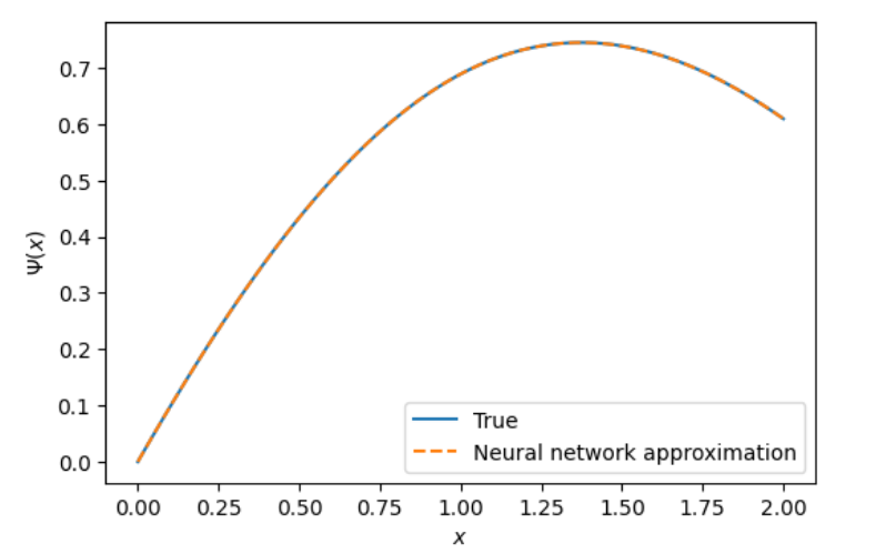
This was a pretty good approximation!! This method can be easily extrapolated to second order. Let’s try it with the next example.

Let’s enforce the Dirichlet boundary conditions.

The trial solution will be changed such that it satisfies BC and reform it in Neural Net.

Theta is a parameter with x as input. N is a neural net with Psi hat as a trial solution. We will use the previous network as it is.

N = nn.Sequential(nn.Linear(1, 50), nn.Sigmoid(), nn.Linear(50,1, bias=False))

Boundary conditions –

A = 0.
B = 0.

Trial solution –

Psi_t = lambda x: A*(1-x) + B * x + (1-x)* x * N(x)

with right-hand side function as -1

f = lambda x, Psi: -1

While in the previous problem we used loss function based directly on the initial equation of first order. This idea is implemented in second-order as well.

Now on implementation, we would need to calculate the second-order derivative. This is easily achieved using Pytorch’s autograd.

def loss(x):

    x.requires_grad = True
    outputs = Psi_t(x)

    #we need Psi_x_x 
    #calculating gradient twice 

    Psi_t_x = torch.autograd.grad(outputs, x, grad_outputs=torch.ones_like(outputs),
                                            create_graph=True)[0]
    Psi_t_x_x = torch.autograd.grad(Psi_t_x, x, grad_outputs=torch.ones_like(Psi_t_x),
                                            create_graph=True )[0]

    return torch.mean((Psi_t_x_x - f(x, outputs)) ** 2)

Using BFGS as optimizer (Adam can also be used)

optimizer = torch.optim.LBFGS(N.parameters())
x = torch.Tensor(np.linspace(0, 1, 100)[:, None])

Running the optimizer

def closure():
    optimizer.zero_grad()
    l = loss(x)
    l.backward()
    return l

for i in range(10):
    optimizer.step(closure)

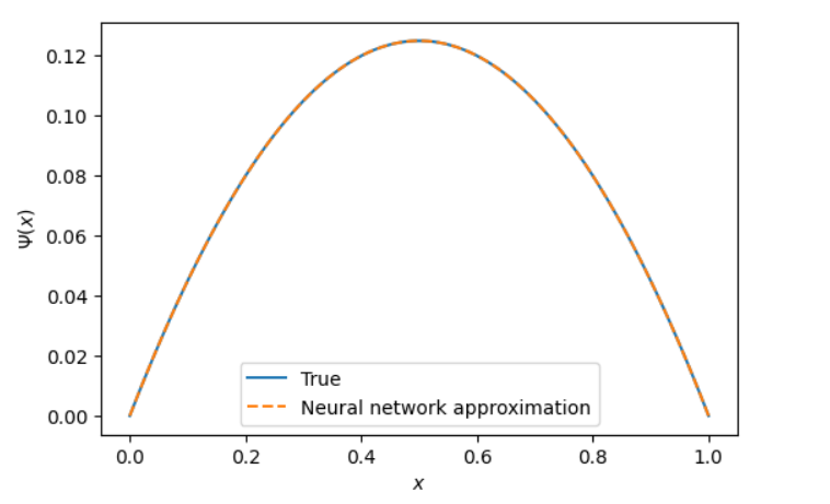
Now we are all done, let’s head to compare our results with the NN approximator.

xx = np.linspace(0, 1, 100)[:, None]

with torch.no_grad():
    yy = Psi_t(torch.Tensor(xx)).numpy()

yt = (0.5) * (-xx**2 + xx ) #actual function pts

fig, ax = plt.subplots(dpi=100)
ax.plot(xx, yt, label='True')
ax.plot(xx, yy, '--', label='Neural network approximation')
ax.set_xlabel('$x$')
ax.set_ylabel('$Psi(x)$')
plt.legend(loc='best');

Conclusion

Results are exactly what we expected for it to be!! Our Network was able to create a function that matches our data points and can be used as a proxy for the analytic solution with minimum errors.

What if we want to extend this idea to PDE (Non-Linear)? There is an excellent paper by George Em Karniadakis – (Physics informed Deep Learning, Solutions of Nonlinear Partial Differential Equations).

Thanks for reading this article! I hope it helped you in realizing how powerful the Neural Network function approximator is for real-life use.

In case of any doubt, reach out to me via LinkedIn (Nihal Singh)

The media shown in this article are not owned by Analytics Vidhya and are used at the Author’s discretion.