Exploratory Data Analysis on UBER Stocks Dataset

This article was published as a part of the Data Science Blogathon

What is EDA(Exploratory data analysis)?

Exploratory data analysis is a great way of understanding and analyzing the data sets. The EDA technique is extensively used by data scientists and data analysts to summarize the main characteristics of data sets and to visualize them through different graphs and plots. It helps data scientists to search for patterns, spot anomalies, or check assumptions. It helps to determine if the statistical techniques that you are using for data analysis are either appropriate or not.

EDA ensures that results are valid and applicable as per the business goals. Once the EDA task is completed, its features can be used for efficient and better data analysis, modelling, and machine learning.

Understanding the dataset

In this article, we are going to perform exploratory data analysis on a small and interesting dataset. The dataset is the UBER stocks dataset that contains seven records, including date, opening value of the stock, closing value of the stock, high and low values of stock that day, the adjacent closing value of the stock, and the volume of stocks that had been traded that day. The dataset consists of 605 records. You can download the dataset from here.

data = pd.read_csv("UBER.csv")
data.head()

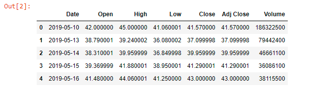
From the above image, you can have a look how the dataset looks like. You can use data.head(x) too, where x represents the number of records you want to see.

Let’s get more insights about the data using pandas ‘describe’ functionality.

data.describe()

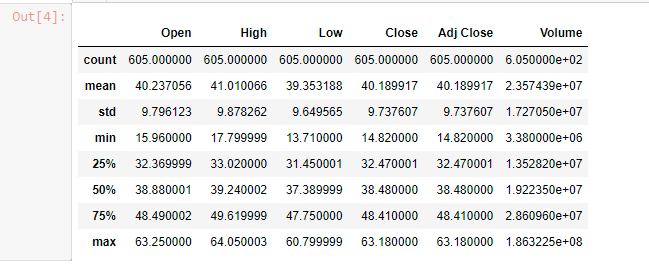
From the above table, we can get several insights into the dataset. We can know a lot of useful information from the above table such as mean, standard deviation, value counts, and how often a value occurs in the dataset.

Prior to doing EDA, we need to check if the dataset contains any null values or not. Our dataset doesn’t contain any values. However, for the sake of curiosity, we will see how the plot would look like if it had null values. We will drop some values from the volume column and we’ll see the results. For that, we will be using the seaborn library.

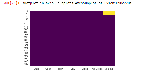
The above image shows that the volume column contains around 25 null values. You can plot the original data frame to see how a dataset without null values would look like.

You can get more information about the data set variables by plotting a heat map.

Heatmap – A heatmap is a 2d representation of data that tells how much a variable is correlated to other variables. It contains values from -1 to 1. Suppose two variables x and y. Let us see the possible causes.

1. When the correlation between x and y is -1, that means x has a negative correlation with y. It simply means when the value of x increases, the value of y would decrease. The more the value is close to -1, the more will be the negative correlation.
2. When the correlation between x and y is 0. It means that x and y have no correlation and are independent.
3. When the correlation between x and y is 1, that means x has a positive correlation with y. Or simply, we can say whenever x increases, y increases too.

Now we know a little about heatmaps, we can proceed towards creating the heatmap on our UBER stocks dataset using the seaborn library.

plt.figure(figsize=(7,5))
sns.heatmap(data.corr(),cmap='Blues',annot=True)

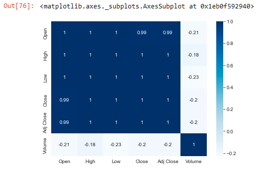
From the above heatmap, you can see a large number of 1s and values close to 1. This means those variables show high positive correlations and are interrelated. This might be possible because of the comparatively very small difference between those values. However, in-stock market this small value is what makes the difference. So, what we are going to do, is add new variables to our dataset that represents the difference between those values.

data['open-high'] = data['Open']-data['High']
data['open-low'] = data['Open'] - data['Low']
data['close-high'] = data['Close']-data['High']
data['close-low'] = data['Close'] - data['Low']
data['high-low'] = data['High'] - data['Low']
data['open-close'] = data['Open'] - data['Close']
data.head()

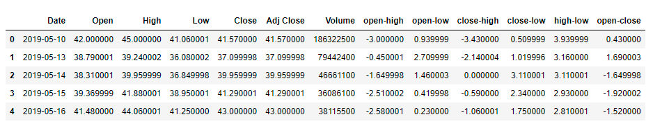
We have added 6 new entries to our dataset. We can now create a heatmap with these new values and see their inter-correlation.

From the previous heatmap, we could realize that those values aren’t very useful. So for more clarity, we will drop those values and take only the new values for creating the heatmap.

data2 = data.copy()
data2 = data2.drop(['Open','High','Low','Close', 'Adj Close'],axis=1)
plt.figure(figsize=(7,5))
sns.heatmap(data2.corr(),cmap='Blues',annot=True)

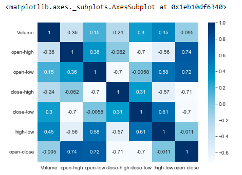
Does this heatmap look more informative than the previous one? I hope you think that too. Based on the correlation values only we can derive several insights for this dataset.

The stock market is all about numbers. Understanding these numbers and finding the pattern is an art, and we the data analysts are the artists. The main variable we are going to focus on in this dataset is the ‘Volume’. Variables having a large correlation value with volume represent that those numbers might have intrigued a large number of buyers and sellers. Correlation between those features and the volume feature will tell us how a change in that feature impacts the number of stocks traded that day.

The open-high shows the most negative correlation with the volume feature. This means that the greater the difference between the opening value of the stock and the highest value of stock that day, the greater will be the stocks traded that day. As there is no information about the number of buyers and sellers, we can only guess that a high difference in opening and highest value of the stock might attract more buyers. Whereas a fewer difference may attract more sellers.

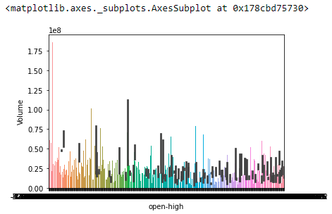
From the below graph, you can observe that the volume is high for smaller values of open-high as compared to larger values of open-high.

sns.barplot(data=data, x = "open-high", y="Volume")

The ‘high-low’ feature shows the maximum value of correlation with the ‘volume’ feature. Thus we can think that a greater fluctuation in the stock price may be a reason behind more transactions of stocks that day.

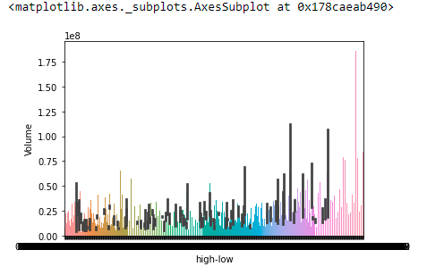
From the below graph you can observe the volume of stocks traded is high for larger values of high-low.

sns.barplot(data=data, x = "high-low", y="Volume")

Conclusion

Exploratory data analysis is an important task in data analysis and helps in better understanding the dataset. It is a necessary step before creating a machine learning model as it helps to understand the relation between variables. Properly done EDA provides a strong base for the overall process, ensures better results, and justifies assumptions with the help of interesting graphs and plots. In this article, we tried to perform EDA on one small but interesting dataset.

I hope you enjoyed reading this article.

Thank you

Also, check the rest of my articles at https://www.analyticsvidhya.com/blog/author/ayush417/

Connect me on LinkedIn – https://www.linkedin.com/in/ayush-gupta-5b9091174/