HQL or Hive Query Language is a simple yet powerful SQL like querying language which provides the users with the ability to perform data analytics on big datasets. Owing to its syntax similarity to SQL, HQL has been widely adopted among data engineers and can be learned quickly by people new to the world of big data and Hive.
In this article, we will be performing several HQL commands on a “big data” dataset containing information on customers, their purchases, InvoiceID, their country of origin and many more. These parameters will help us better understand our customers and make more efficient and sound business decisions.

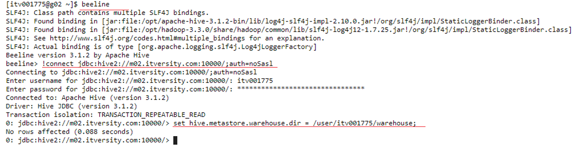
For the purpose of execution, we would be using Beeline command Line Interface which executes queries through HiveServer2.
Next, we type in the following command which connects us to the HiveServer2.
!connect jdbc:hive2://m02.itversity.com:10000/;auth=noSasl
It requires authentication so we input the username and password for this session and provide the location or path where we have our database stored. The commands(underlined in red) for this are given below.
set hive.metastore.warehouse.dir = /user/username/warehouse;
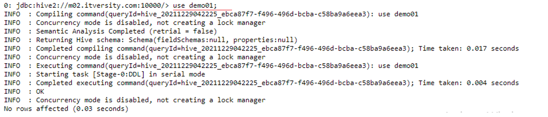
Now that we are connected to HiveServer2 we are ready to start querying our database. Firstly we create our database “demo01” and then type in the command to use it.
Use demo01;
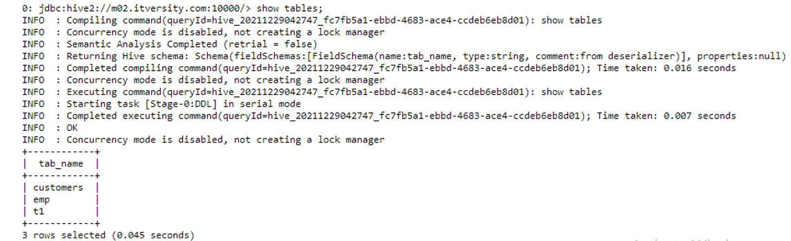
Now we are going to list all the tables present in the demo01 database using the following command
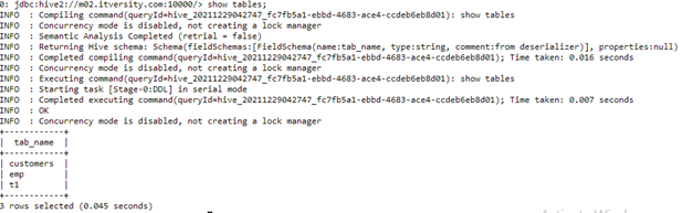
show tables;
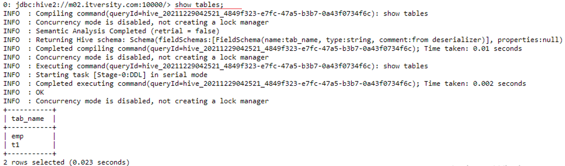
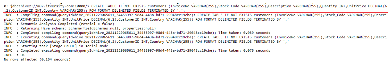
As we can see above 2 tables “emp” and “t1” are already present in the demo01 database. So for our customer’s dataset, we are going to create a new table called “customers”.
CREATE TABLE IF NOT EXISTS customers (InvoiceNo VARCHAR(255),Stock_Code VARCHAR(255),Description VARCHAR(255),Quantity INT,UnitPrice DECIMAL(6,2),CustomerID INT,Country VARCHAR(255)) ROW FORMAT DELIMITED FIELDS TERMINATED BY ',' ;
Now if we run the “show tables” command we see the following output.
We can see that a table named customers has been created in the demo01 database. We can also see the schema of the table using the following command.
desc customers;
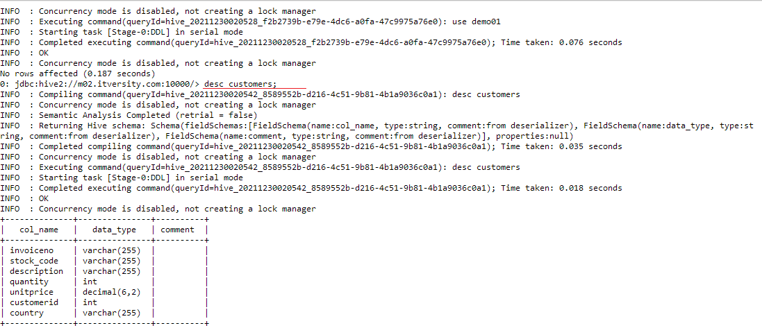
Now we upload our new.csv file containing customer records to our hdfs storage using this command.
hdfs dfs -put new.csv /user/itv001775/warehouse/demo01.db/customers

Now we have to load this data into the customer’s table we created above. To do this we run the following command.
load data inpath
'/user/itv001775/warehouse/demo01.db/customers/new.csv' into table customers;
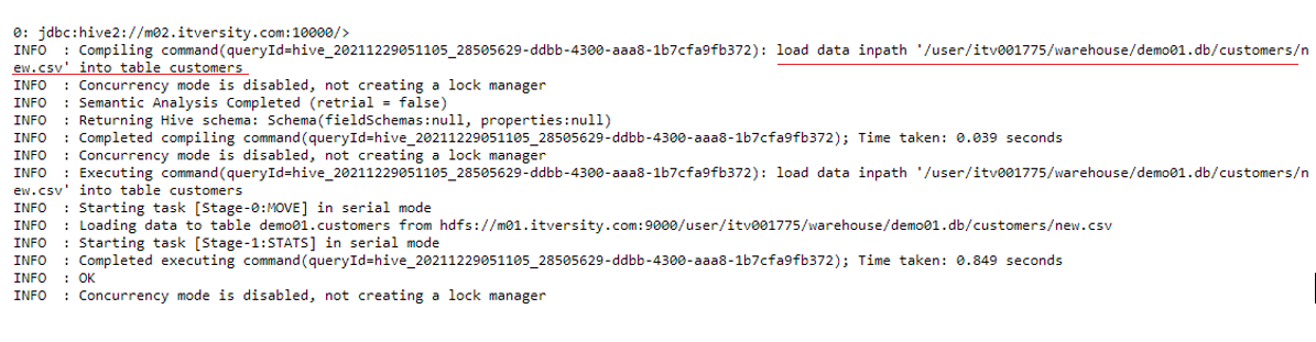
This concludes the part where we have uploaded the data on hdfs and loaded it into the customer’s table we created in the demo01 database.
Now we shall do a bit of data eyeballing meaning to have a look at the data and see what insights can be extracted from it. As the dataset contains over 580,000 records we shall have a look at the first 5 records for convenience using this command.
select * from customers limit 5;
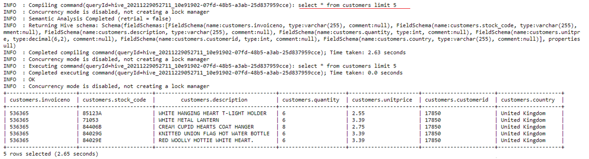
We can see above it has 7 columns namely invoiceno, stock_code, description, quantity, unitprice, customerid and country. Each column brings value and insights for the data analysis we are going to perform next.
DATA ANALYSIS THROUGH HQL
CASE 1: We want to insert
into customers table the records of a customer from Germany with customerid- 18443 who bought a Gaming PC, invoice number 610221,
stock code 3427AB, quantity 2 at a unit price of 9000.
QUERY:
insert into customers values (‘610221’,’3427AB’,’Gaming PC’,2,9000,18443,’Germany’);
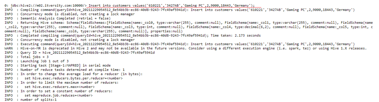
Now we can query the database to see if the record was inserted successfully.
select * from customers limit 5;
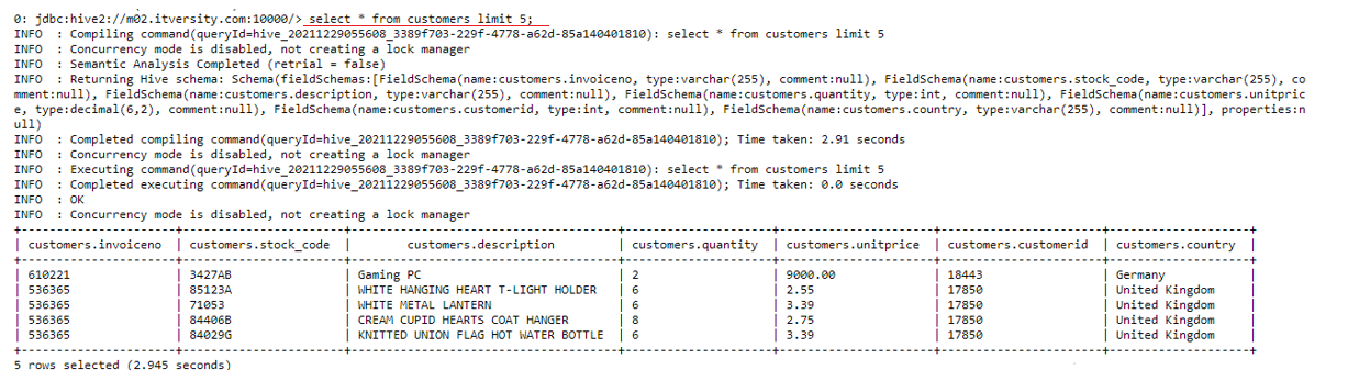
As we can see record has been inserted.
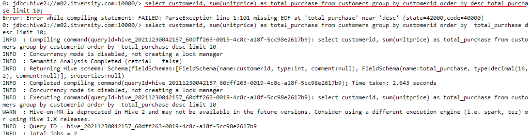
CASE 2: We want to see the sum of the purchases made by each customer along with invoiceno in descending order.
QUERY: (for convenience we limit our output to the first 10 records)
select customerid, sum(unitprice) as total_purchase from customers group by customerid order by total_purchase desc limit 10;
In the above query, we are grouping our records together based on the same customers id’s and ordering the results by total purchase made by each customer.
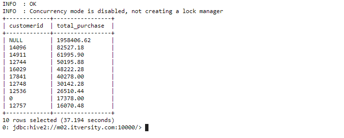
Apart from the customers without a customerid, we are able to find out our top 10 customers according to the amount of their purchase. This can be really helpful in scouting and targeting potential customers who would be profitable for businesses.
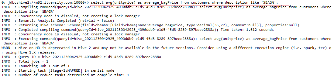
CASE 3: We want to find out the average price of bags being sold to our customers.
QUERY:
select avg(unitprice) as average_bagPrice from customers where description like '%BAG%';
Note that in the above query we used the “like” logical operator to find the text from the description field. The “%” sign represents that anything can come before and after the word “bag” in the text.
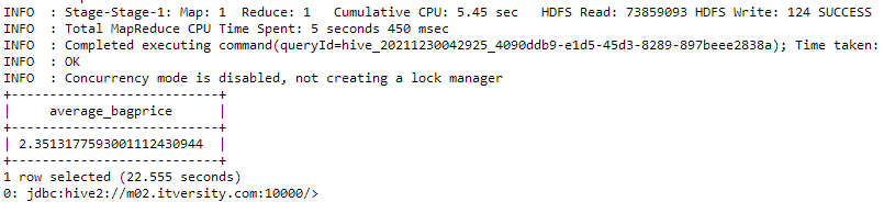
We can observe that the average price across the spectrum of products sold under the tag of bags is 2.35(dollars, euros or any other currency). The same can be done for other articles which can help companies to determine the price ranges for their products for better sales output.
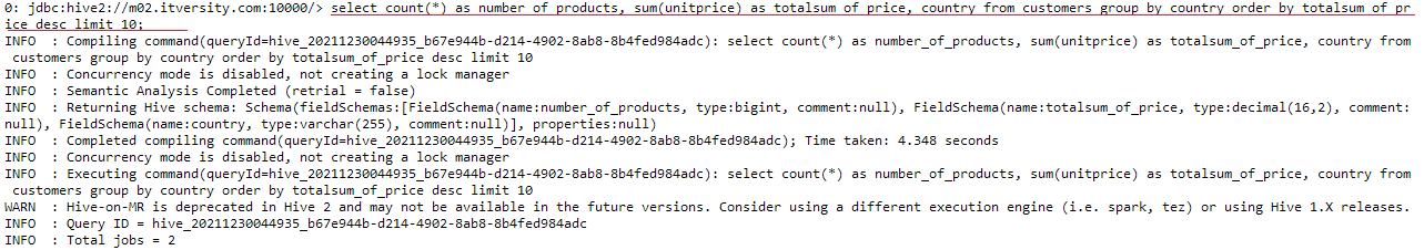
CASE 4: We want to count the number of products sold and the average
price of products for top 10 countries in descending order by count.
QUERY:
select count(*) as number_of_products, sum(unitprice) as totalsum_of_price, country from customers group by country order by totalsum_of_price desc limit 10;
Here count(*) means counting all the records separately for each country and ordering the output by total sum of price of goods sold in that country.
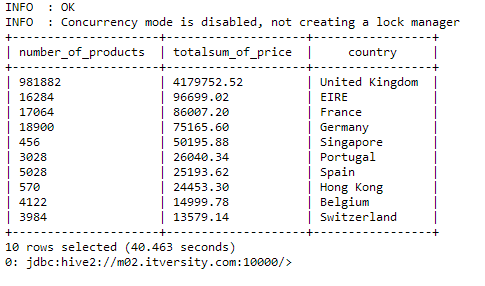
Through this query, we can infer the countries the businesses should target the most as the total revenue generated from these countries is maximum.
CASE 5: display the customerid and total number of products ordered for each
customer having quantity greater than 10, ordered in descending according to
quantity for top 20 customers.
QUERY:
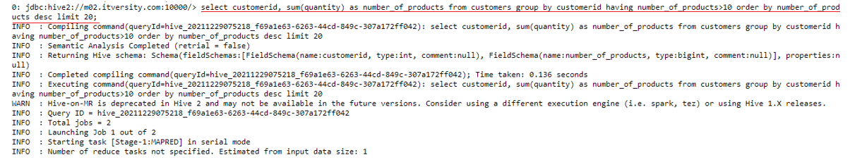
select customerid, sum(quantity) as number_of_products from customers group by customerid having number_of_products>10 order by number_of_products desc limit 20;
For each customer, we are grouping their records by their id and finding the number of products they bought in descending order of that statistic. We also employ the condition that only those records are selected where a number of products are greater than 10.
Note that we always use the “having” clause with the group by when we want to specify a condition.
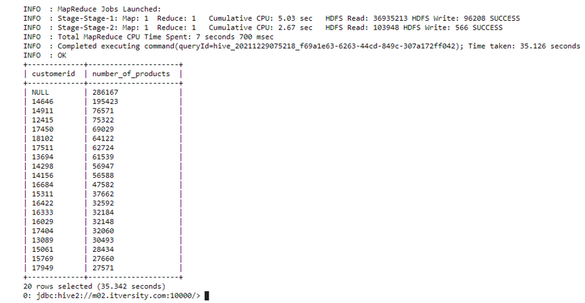
Through this, we can see our top customers based on the number of products they ordered. The customers ordering the most generate the most amount of profit for the company and thus should be scouted and pursued the most, and this analysis helps us find them efficiently.
BONUS
Hive has an amazing feature of sorting our data through the “Sort by” clause. It almost does the same function as the “order by” clause as in they both arrange the data in ascending or descending order. But the main difference can be seen in the working of both these commands.
We know that in Hive, the queries we write in HQL are converted into MapReduce jobs so as to abstract the complexity and make it comfortable for the user.
So when we run a query like :
Select customerid, unitprice from customers sort by customerid;
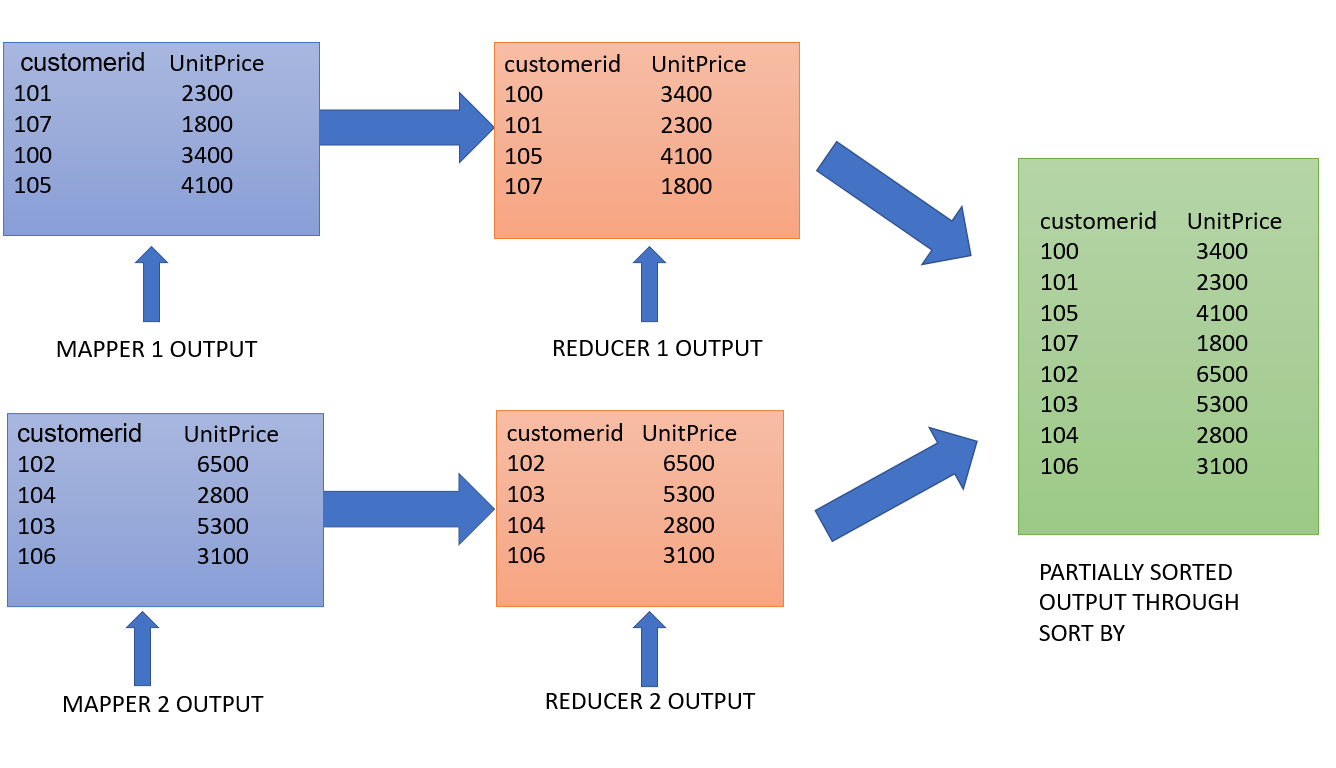
Multiple mappers and reducers are deployed for the MapReduce job. Give attention to the fact that multiple reducers are used which is the key difference here.
Multiple mappers output their data into their respective reducers where it is sorted according to the column provided in the query, customerid in this case. The final output contains the appended data from all the reducers, resulting in partial sorting of data.
Whereas in order by multiple mappers are used along with only 1 reducer. Usage of a single reducer result in complete sorting of the data passed on from the mappers.
Select customerid, unitprice from customers order by customerid;
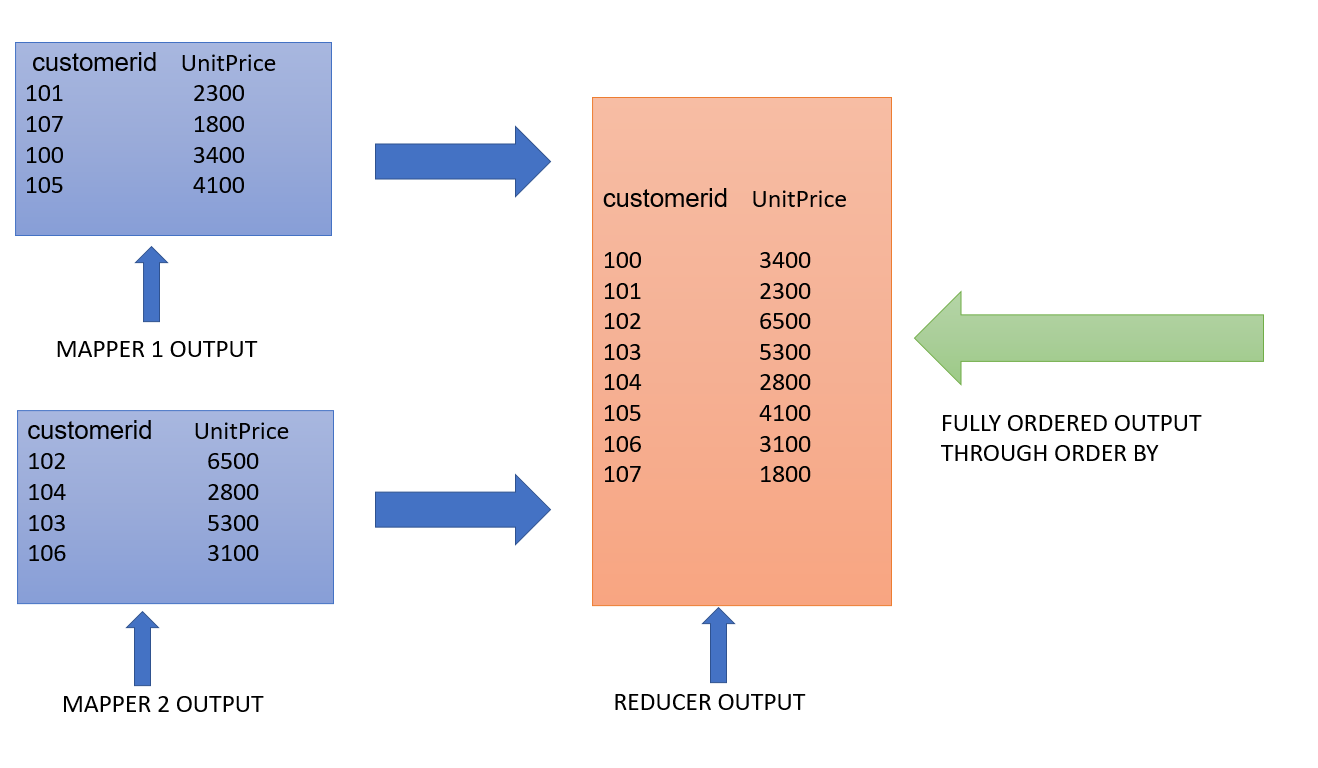
The difference in the Reducer output can be clearly seen in the data. Hence we can say that “order by” guarantees complete order in the data whereas “sort by” delivers partially ordered results.
ENDNOTES
In this article, we have learned to run HQL queries and draw insights from our customer dataset for data analytics. These insights are valuable business intelligence and are very useful in driving business decisions.
If you have any questions related to how HQL commands for data analytics do let me know in the comments section below.
Read more articles on Data Analytics here.


