This article was published as a part of the Data Science Blogathon.
The real estate business manages large amounts of data and information. Real Estate agents need to take in a lot of factors before deciding the price of a building, a flat, or a house. Real estate and property prices are affected by a lot of factors. A home closer to the city centre will cost more than a house far away from the city. Understanding and determining real estate prices requires a lot of data.

(Image Source: https://www.pexels.com/photo/aerial-view-of-white-concrete-buildings-during-golden-hours-681368/)
Factors affecting Real Estate Prices
One of the most critical factors affecting the price of a house or flat is the location. A flat in Kolkata or Delhi will cost more than a flat in Indore or Bhopal. Similarly, properties located in the market or commercial areas are costlier than properties in the suburbs or away from commercial areas. Property costs rely upon the presence of neighbouring municipal conveniences. Properties having schools, markets, shops, hospitals, etc., close to them will have higher prices.
The cost of properties is also dependent on the mean of pay of people in that area. That’s why properties have higher values in industrial, commercial areas, and IT hubs and individuals will often have higher salaries around there and have higher spending limits.
The prices of the property also depend upon supply and demand. In dense metropolitan cities, there is a lack of property due to lack of land. In such places, the property price will be high due to the high demand for property. But the availability of living and commercial space is low, owing to less land availability.
We can analyze existing real estate prices to predict the price of real estate. This can be very useful in understanding the valuation of a property or a new development. We shall use some sample real estate data to predict real estate prices.
Many people get confused about the prices while purchasing a property. Often, they end up paying too much for a flat or a house.
The Data
The data belongs to real estate properties in Taipei, Taiwan. Taipei is a prime metropolitan city with many high tech companies, and real estate prices will tend to be on the higher side in Taipei. The data consists of 7 features, out of which six will be input features, and one will be the output feature.
The features are
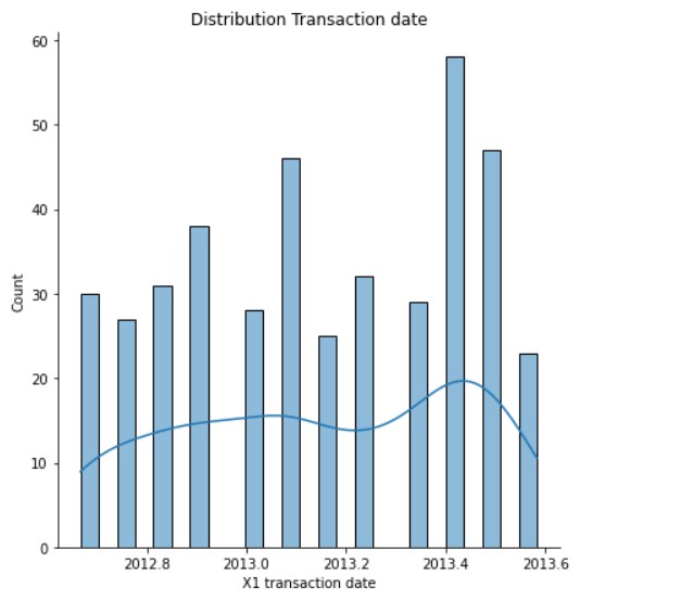
Transaction date: The date of the real estate transaction. Here, an important thing that should be pointed out is that the date is a decimal of the whole year, and that is, say 1st July 2012 would be 2012.500. This is an exciting way to put the date data.
House age: The house age in years. The age of a house can determine its price. Newer properties tend to have higher fees than older ones. Similarly, older homes can be found cheaper.
Distance to the nearest MRT station: MRT or Mass Rapid Transit, usually means the Metro Rail system in large cities. People use these systems for transportation and going to the office. Houses near MRT stations are bound to have higher prices than those far away from them. Proximity to metro stations helps commuters, and they can easily travel from one place to another. It increases the convenience of people. MRT stations usually connect all the essential parts of a city. Fast and rapid transport makes the office commute easy.
The number of nearby Convenience Stores: Close by stores are significant for any home or property. The quantity of neighbouring stores or grocery stores is essential in choosing land cost. When individuals can get the necessities they need effectively; the property furnishes them with higher worth. Along these lines, a property with more stores nearby will probably have higher costs.
Latitude and Longitude: These features might relate to the prices, which might not be visible on a direct view. We will plot them on the map to understand the distribution of the properties.
House price (per unit area): This is the actual price of the house (per unit area). We will need to predict this feature based on other parts, and costlier properties will have higher values and vice versa.
Getting Started
First, we import the necessary libraries.
import numpy as np
import pandas as pd
import matplotlib.pyplot as plt
%matplotlib inline
import seaborn as sns
The primary libraries we will need to perform analysis are imported. Now, we read the data.
df = pd.read_csv('Real estate.csv')
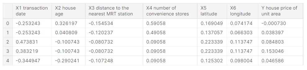
df.head()
Output:
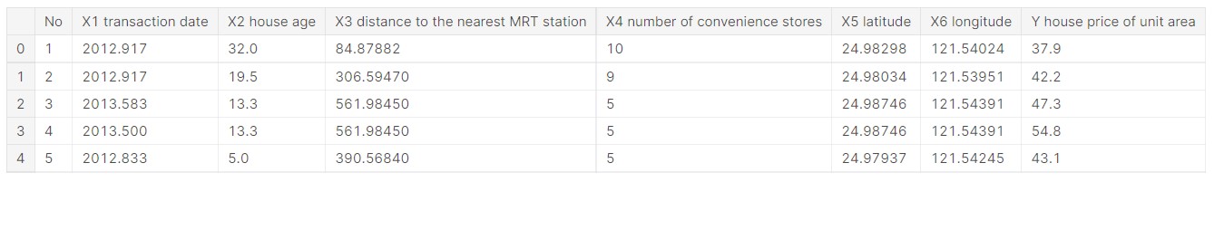
Now, we have an overview of how the data looks.
Let us check what columns are present in the data.
df.columns
Output:
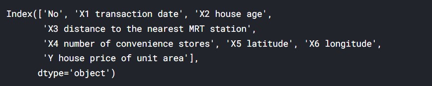
(Source: Author)
Now, we check the data information.
df.info()
Output:
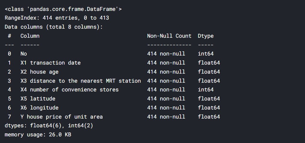
(Source: Author)
Let us now check for missing values.
#Checking for missing data
df.isna().sum()
Output:

(Source: Author)
Let us plot the distribution plots of all the data to understand the data.
Distribution of House Price ( Per Unit Area )
sns.displot(data= df, x='Y house price of unit area' , bins=25 , kde=True, height=6)
plt.title("Distribution of House Price per Unit Area")
Output:
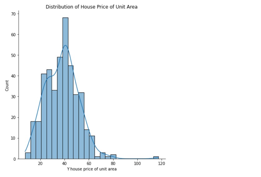
(Source: Author)
Distribution Transaction date
sns.displot(data= df, x='X1 transaction date' , bins=25 , kde=True, height=6)
plt.title("Distribution Transaction date")
Output:
(Source: Author)
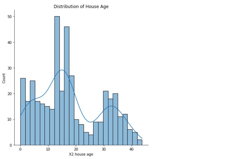
Distribution of House Age
sns.displot(data= df, x='X2 house age' , bins=25 , kde=True, height=6)
plt.title("Distribution of House Age")
Output:
(Source: Author)
So, here we can see that the house ages have a wide distribution.
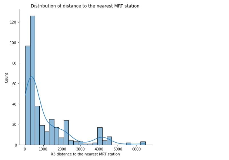
Distribution of distance to the nearest MRT station
sns.displot(data= df, x='X3 distance to the nearest MRT station' , bins=25 , kde=True, height=6)
plt.title("Distribution of distance to the nearest MRT station")
Output:
(Source: Author)
This distance is in metres, so we can see that most properties are in 1km to 2km of MRT stations. But, a few properties are very far away.
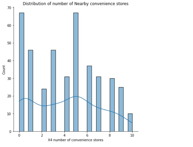
Distribution of the number of Nearby convenience stores
sns.displot(data= df, x='X4 number of convenience stores' , bins=25 , kde=True, height=6)
plt.title("Distribution of number of Nearby convenience stores")
Output:
(Source: Author)
There is a good distribution here. A section of properties has few convenience stores nearby, while others have many.
Distribution of Latitude
sns.displot(data= df, x='X5 latitude' , bins=25 , kde=True, height=6)
plt.title("Distribution of latitude")
Output:
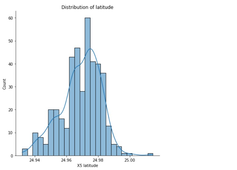
(Source: Author)
Distribution of Longitude
sns.displot(data= df, x='X6 longitude' , bins=25 , kde=True, height=6)
plt.title("Distribution of longitude")
Output:
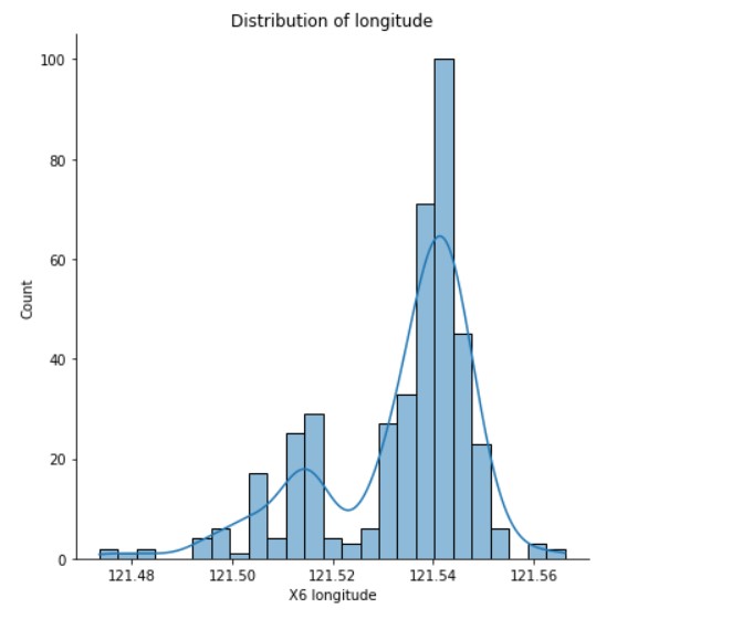
(Source: Author)
We plot the locations on the map using the latitude and longitude data.
For this, we first import Folium.
#plotting on map
import folium
from folium import Choropleth, Circle, Marker
from folium.plugins import HeatMap, MarkerCluster
Now, we create a map to analyze the location of the properties. The reference point of the map will be the mean of the data distribution of latitude and longitude. We shall be using the style “Stamen Toner”.
# Create a map
city= folium.Map(location=[24.98, 121.52], tiles='Stamen Toner', zoom_start=12)
city
Output:
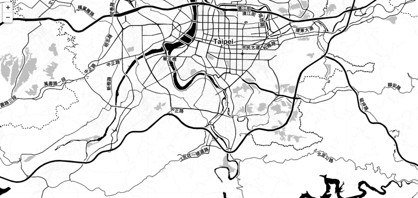
(Source: Author)
Here, we get the map view of Taipei. Now, we need to plot the properties on the map.
for i in range (0,len(df)):
    lat=df["X5 latitude"][i]
    long=df["X6 longitude"][i]
    folium.Marker(
    [lat, long], ).add_to(city)
city
Output:
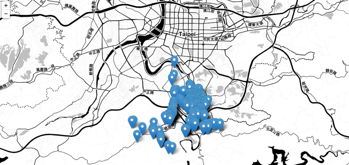
(Source: Author)
Now, we have plotted the real estate properties. We can understand that the properties are in the southern part of Taipei towards the suburbs. The actual map in the notebook is interactive, and I will share the link to the notebooks so that one can see them.
Price Prediction
First, we import the necessary libraries.
import tensorflow as tf
from sklearn.model_selection import train_test_split
from tensorflow.keras.models import Sequential
from tensorflow.keras.layers import Dense, Dropout
from tensorflow.keras.callbacks import EarlyStopping, LambdaCallback
Now, we normalize the data. Normalization in Deep Learning and Machine Learning converts the data into a similar scale. The most common way to normalize data is by scaling the data.
How it works:
X norm = ( X – Xmin)/ (Xmax- Xmin)
This process helps distribute data correctly, and the data is formatted, and outliers are removed.
Let us implement normalization.
df = df.iloc[:,1:]
df_norm = (df - df.mean()) / (df.max()-df.min())
df_norm.head()
Output:
(Source: Author)
So, now we can see that the data is normalized.
Let us see the correlation in the normalized data.
df_norm.corr()
Output:
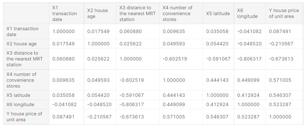
(Source: Author)
The latitude, longitude and number of stores have a high positive correlation, which is very obvious. Many convenience stores nearby will mean a better location and higher real estate prices.
Similarly, house age and distance to MRT station have a high negative correlation, and this indicates that a lower house age and low distance to MRT station means the property will have higher prices.
We create a function to get the predicted house price in the average costs, which will negate the normalization.
#converting back the normalized price to real value of price
y_mean = df['Y house price of unit area'].mean()
y_std = df['Y house price of unit area'].std()
def convert_label_value(pred):
    return int(pred * y_std + y_mean)
We test the function now.
#testing the function
print(convert_label_value(0.12))
Output:
39
Now, we create the training and testing sets of data.
Creating Training and Testing sets
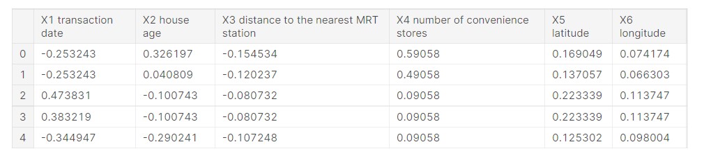
#input features
X = df_norm.iloc[:, :6]
X.head()
Output:
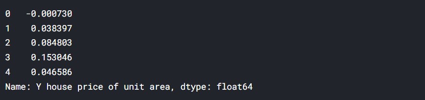
# y value
y = df_norm.iloc[:, -1]
y.head()
Output:
#Feature and label values
X_arr = X.values
y_arr = y.values
X_train, X_test, y_train, y_test = train_test_split(X_arr, y_arr, test_size = 0.2, shuffle = True, random_state=7)
print('X_train shape: ', X_train.shape)
print('y_train shape: ', y_train.shape)
print('X_test shape: ', X_test.shape)
print('y_test shape: ', y_test.shape)
Output:
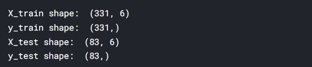
The data has been split successfully.
Creating the Model
We shall be creating a neural network model to perform the training, and it will be a sequential model.
We are creating a simple model with four layers.
def get_model():
    model = Sequential([
        Dense(5, input_shape = (6,), activation = 'relu'),
        Dense(12, activation = 'sigmoid'),
        Dense(6, activation = 'relu'),
        Dense(1)
    ])
    model.compile(
        loss='mse',
        optimizer='adadelta'
    )
    return model
model = get_model()
model.summary()
Output:
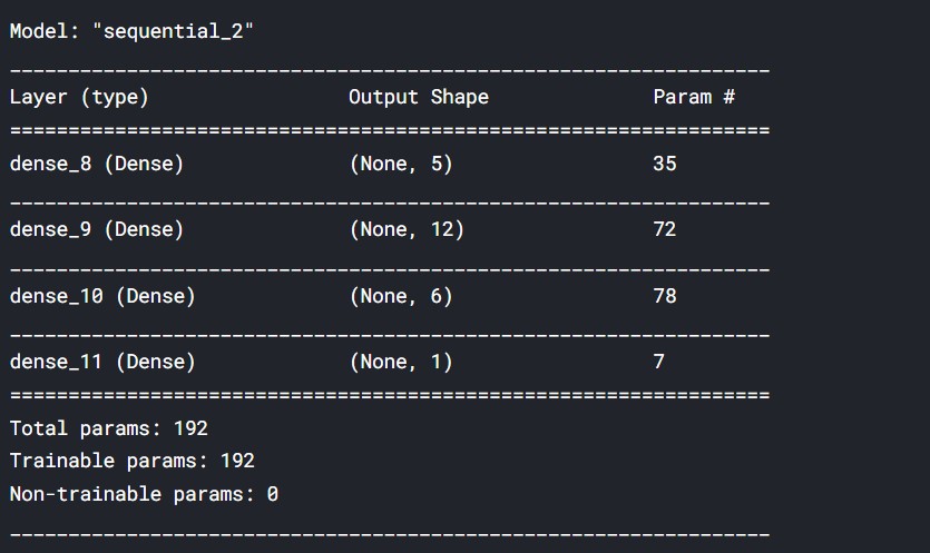
(Source: Author)
Our Model is ready now. We will train the data into the Model.
Training the Model using Train data
Now, we shall introduce the Model using our data.
early_stopping = EarlyStopping(monitor='accuracy', patience = 5)
history = model.fit(
    X_train, y_train,
    validation_data = (X_test, y_test),
    epochs = 100,
    callbacks = [early_stopping]
)
Initial and final steps:
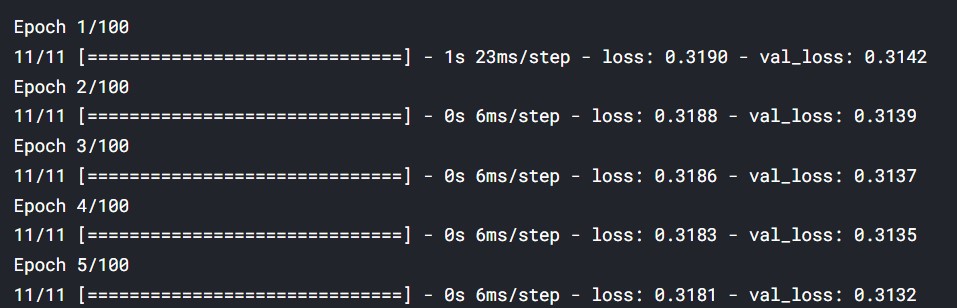
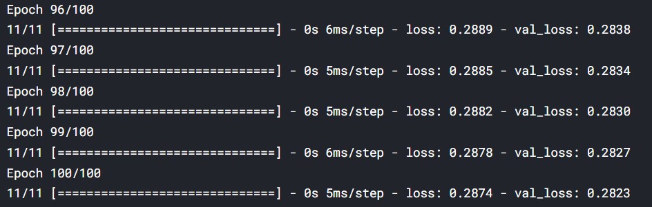
(Source: Author)
I will share the link to the entire notebook.
Sample Values
Now, we shall be taking a sample value and making a test prediction to understand the Model’s performance. Let us get started.
For the time of the transaction, we are taking the midpoint of 2012.
#Take the year of sale
date=2012.500
date=(date- mean_val[0] )/ std_val[0]
We are taking the age of the house: 23 years.
#Take house age in years
age= 23
age= (age- mean_val[1] )/ std_val[1]
We take the distance to the nearest metro station = 1200.
#Distance to nearest metro staion (in m)
mrt= 1200
mrt= (mrt- mean_val[2] )/ std_val[2]
We are taking the number of stores to be 5.
#number of stores in the locality
stores=5
stores=(stores- mean_val[3] )/ std_val[3]
Standard latitude and longitude values.
#latitude
latitude=24.97
latitude=(latitude- mean_val[4] )/ std_val[4]
#longitude
longitude=121.53
longitude=(longitude- mean_val[5] )/ std_val[5]
Test Prediction
Now, we perform a test prediction.
#numpy array
test_input= np.array( [[ date, age, mrt, stores, latitude, longitude]] )
#prediction
val= model.predict(test_input)
res=val[0][0]
#testing the function
print("The predicted price is=",convert_label_value(res))
Output:
The predicted price is= 32
When we perform the prediction, we are getting a realistic price. This means the Model functions correctly and can give a projection from the training data.
( All code outputs are credits of the author).
Conclusion
Real Estate price prediction using a sequential model is an interesting topic, and we used data to analyze real estate prices and understand the reason behind these. Multiple factors determine such prices, and using a large amount of data can be an excellent way to perform predictive analytics and make predictions. Deep Learning and ML have a lot of applications in real life, and we had a look at one of these applications.
Proper predictive models and be of immense use to both real estate sellers and buyers.
The code used :
Thank You.
Read another article based on the sequential model on our blog!
The media shown in this article is not owned by Analytics Vidhya and are used at the Author’s discretion.
Prateek is a dynamic professional with a strong foundation in Artificial Intelligence and Data Science, currently pursuing his PGP at Jio Institute. He holds a Bachelor's degree in Electrical Engineering and has hands-on experience as a System Engineer at TCS Digital, where he excelled in API management and data integration. Prateek also has a background in product marketing and analytics from his time with start-ups like AppleX and Milkie Way, Inc., where he was involved in growth campaigns and technical blog management. Recognized for his structured thinking and problem-solving abilities, he has received accolades like the Dr. Sudarshan Chakraborty Award for Best Student Performance. Fluent in multiple languages and passionate about technology, Prateek continues to expand his expertise in the rapidly evolving AI and tech landscape.


